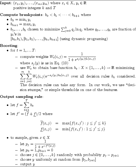
Having described how we set up the learning problem, we are now ready to describe the learning algorithm that we used. Briefly, we solved this learning problem by first reducing to a multiclass, multi-label classification problem (or alternatively a multiple logistic regression problem), and then applying boosting techniques developed by Schapire and Singer SchapireSi99,SchapireSi00 combined with a modification of boosting algorithms for logistic regression proposed by Collins, Schapire and Singer CollinsScSi02. The result is a new machine-learning algorithm for solving conditional density estimation problems, described in detail in the remainder of this section. Table 5 shows pseudo-code for the entire algorithm.
Abstractly, we are given pairs
![]() where each
where each
![]() belongs to a space
belongs to a space ![]() and each
and each ![]() is in
is in
![]() .
In our case, the
.
In our case, the ![]() 's are the auction-specific feature vectors
described above; for some
's are the auction-specific feature vectors
described above; for some ![]() ,
,
![]() . Each target quantity
. Each target quantity
![]() is the difference between
closing price and current price.
Given a new
is the difference between
closing price and current price.
Given a new ![]() , our goal is to estimate the conditional distribution
of
, our goal is to estimate the conditional distribution
of ![]() given
given ![]() .
.
We proceed with the working assumption that all training and test
examples ![]() are i.i.d. (i.e, drawn independently from identical
distributions).
Although this assumption is false in our
case (since the agents, including ours, are changing
over time), it seems like a reasonable approximation that greatly
reduces the difficulty of the learning task.
are i.i.d. (i.e, drawn independently from identical
distributions).
Although this assumption is false in our
case (since the agents, including ours, are changing
over time), it seems like a reasonable approximation that greatly
reduces the difficulty of the learning task.
Our first step is to reduce the estimation problem to a classification
problem by
breaking the range of the ![]() 's into bins:
's into bins:
For each of the breakpoints ![]() (
(![]() ),
our learning algorithm attempts to
estimate the probability that a new
),
our learning algorithm attempts to
estimate the probability that a new ![]() (given
(given ![]() ) will be at least
) will be at least
![]() .
Given such estimates
.
Given such estimates ![]() for each
for each ![]() , we can then estimate the
probability that
, we can then estimate the
probability that ![]() is in the bin
is in the bin ![]() by
by ![]() (and we can then use a constant density within each bin).
We thus have reduced the problem to one of estimating multiple
conditional Bernoulli
variables corresponding to the event
(and we can then use a constant density within each bin).
We thus have reduced the problem to one of estimating multiple
conditional Bernoulli
variables corresponding to the event ![]() , and for this, we use
a logistic regression algorithm based on boosting techniques as
described by CollinsScSi02 CollinsScSi02.
, and for this, we use
a logistic regression algorithm based on boosting techniques as
described by CollinsScSi02 CollinsScSi02.
Our learning algorithm constructs a real-valued function
![]() with the interpretation that
with the interpretation that
We attempt to minimize this quantity for all training examples
![]() and all breakpoints
and all breakpoints ![]() .
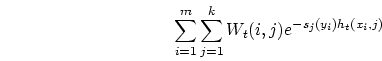
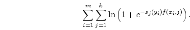
Specifically, we try to find a function
.
Specifically, we try to find a function ![]() minimizing
minimizing
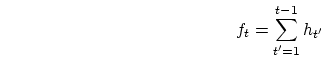
When computed by this sort of iterative procedure,
CollinsScSi02 CollinsScSi02 prove the asymptotic convergence
of ![]() to the minimum of the objective function in
Equation (11) over all linear combinations of the base
functions. For this problem, we fixed the number of rounds to
to the minimum of the objective function in
Equation (11) over all linear combinations of the base
functions. For this problem, we fixed the number of rounds to
![]() . Let
. Let ![]() be the final predictor.
be the final predictor.
As noted above, given a new feature vector ![]() , we compute
, we compute ![]() as in
Equation (9) to be our estimate for the probability that
as in
Equation (9) to be our estimate for the probability that
![]() , and we let
, and we let ![]() and
and ![]() . For this to make
sense, we need
. For this to make
sense, we need
![]() , or equivalently,
, or equivalently,
![]() , a condition that may not
hold for the learned function
, a condition that may not
hold for the learned function ![]() . To force this condition, we
replace
. To force this condition, we
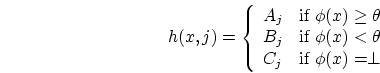
replace ![]() by a reasonable (albeit heuristic) approximation
by a reasonable (albeit heuristic) approximation ![]() that
is nonincreasing in
that
is nonincreasing in ![]() , namely,
, namely,
![]() where
where
![]() (respectively,
(respectively, ![]() ) is the pointwise minimum
(respectively, maximum) of all nonincreasing functions
) is the pointwise minimum
(respectively, maximum) of all nonincreasing functions ![]() that
everywhere upper bound
that
everywhere upper bound ![]() (respectively, lower bound
(respectively, lower bound ![]() ).
).
With this modified function ![]() , we can compute modified
probabilities
, we can compute modified
probabilities ![]() . To sample a single point according to the
estimated distribution on
. To sample a single point according to the
estimated distribution on
![]() associated with
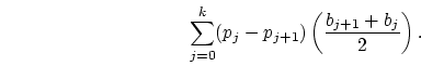
associated with ![]() , we choose bin
, we choose bin
![]() with probability
with probability ![]() , and then select a
point from this bin uniformly at random. Expected value according to
this distribution is easily computed as
, and then select a
point from this bin uniformly at random. Expected value according to
this distribution is easily computed as
Although we present results using this algorithm in the trading agent context, we did not test its performance on more general learning problems, nor did we compare to other methods for conditional density estimation, such as those studied by Stone94 Stone94. This clearly should be an area for future research.