Linear and Integer Programming
Learning Objectives
Formulate a problem as a Linear Program (LP)
Convert a LP into a required form, e.g., inequality form
Plot the graphical representation of a linear optimization problem with two variables and find the optimal solution
Understand the relationship between optimal solution of an LP and the intersections of constraints
Describe and implement a LP solver based on vertex enumeration
Describe the high-level idea of the Simplex (hill climbing) algorithm
Formulate a problem as a Integer or Linear Program (IP or LP)
Write down the Linear Program (LP) relaxation of an IP
Plot the graphical representation of an IP and find the optimal solution
Understand the relationship between optimal solution of an IP and the optimal solution of the relaxed LP
Describe and implement branch-and-bound algorithm
Understand some of the ethical concerns around the high resource cost needed to solve many modern computing problems
Introduction and Formulation
Optimization problems are closely tied with constraint satisfaction problems. The main difference is that optimization problems introduce a notion of cost we'd like to minimize/maximize, whereas with CSPs we are satisfied with any assignment of our variables that will satisfy the constraints.
The first step to finding the solution is to define the variables present in the problem. These variables will be the components used to formulate the cost vector (used in the objective function) and the constraints.
The general format for an LP formulation is as follows: \[\texttt{min}_\mathbf{x} \texttt{ } c^T\mathbf{x}\] \[\texttt{s.t } \mathbf{Ax} \preceq \mathbf{b}\] where:
\(\mathbf{c}\) = the cost vector
\(\mathbf{x}\) = variable vector
\(\mathbf{A}\), \(\mathbf{b}\) = coefficient matrix and vector (respectively) representing the constraints
We can alter any constraint that is not of the form \(\preceq\) to match the rest of the constraints.
Cost Contours
Let's consider the LP cost function \(f(x) = c^Tx\). A cost contour of \(f\) is formally defined as the set of all points \(x'\) such that \(k = f(x')\) for a given \(k\) (for those of you who have taken Calc 3, "cost contour" is synonymous with "level curve"). We can visualize this for \(c = [1\ 3]^T\). This function defines a plane, visualized below. The cost contours will be the lines determined by taking cross sections of the plot of the function at varying \(z\) values (costs).
![A plot of the plane z = x + 3y, corresponding to c = [1\ 3]^T](images/3dcontour.png)
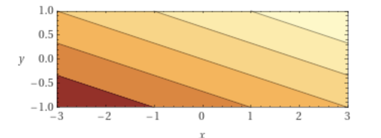
Notice that cost will increase when travelling in the direction of the cost vector, and decrease when going opposite. It follows that since all the points on a contour have the same cost, each contour is perpendicular to the direction of increasing cost defined by cost vector. The vectors for our constraint lines point away from our feasible region, however.
What happens when the magnitude of the cost vector increases? Since the overall change between the cost for the different contours will increase, to compensate for this effect, the contour lines will move closer together. Therefore, the distance between cost contours will decrease.
Algorithms for Solving Linear Programs
Once we have read the problem description, we need to find the solution (if it exists). We are guaranteed that if there is a solution to the LP it will be at one of the feasible intersections of the constraint boundaries. If the feasible region is not enclosed, however, then the solution can become negative infinity.
Now that we have formulated the LP, we can take our cost vector and constraints and use one of the algorithms we have for finding the solution.
There are two main algorithms that we will talk about in this course:
Vertex Enumeration: Check the value of the objective function at all feasible intersections and pick the intersection that has the smallest value (assuming a minimization problem)
Simplex: Start with an arbitrary intersection. Iteratively move to a best neighboring vertex until no better neighbor found
Example
Consider a simple example where the objective function is \(2x_1 + 3x_2\), with 4 constraints: \[-x_2 \leq -1, ~~ x_1+3x_2 \leq 11, ~~ -2x_1+x_2 \leq -1,~~ 2x_1+x_2 \leq 12\] Vertex Enumeration:
Step 1. Evaluate all the values of objective function at all intersections of feasible region
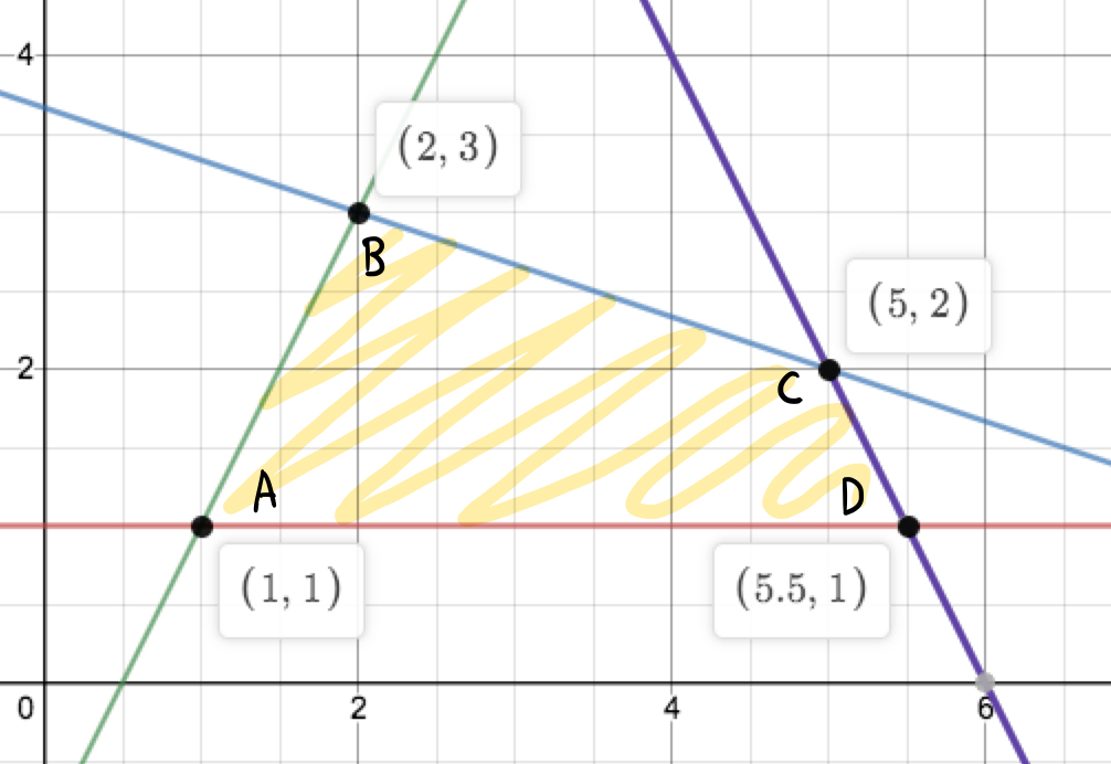 \(A = 2(1) + 3(1) = 5, B = 10, C = 16, D = 14\)
Step 2. Choose the vertex with the smallest value. In this example, it would be vertex A. Hence, \(x_1 = 1, x_2 = 1\).
Simplex:
Step 1. Choose arbitrary vertex and get objective value. Ex, choose \(C = 16\).
Step 2. Evaluate objective values of its neighbors. \(B = 10, D = 14\). If exists, move to best neighboring vertex, in this case B.
Try walking through the rest of the Simplex algorithm yourself!
Algorithm for Solving Integer Programs: Branch and Bound
Now that we have learned how to formulate and solve Linear Programs, we can consider an additional restriction on the solution that all variables must have an integer value. With this new constraint, we now must update the way in which we find the solution.
To solve an Integer Programming problem, we can use the Branch and Bound algorithm:
# IP: a minimization integer program with constraints and objective function cost
def branch_and_bound(IP):
    1. Push LP solution of problem into priority queue (PQ), ordered by minimizing objective value of LP solution
    2. Repeat:
        If PQ is empty, return IP is infeasible

        candidate_sol = PQ.pop() #LP solution x*_LP to a set of constraints c

        If candidate_sol is all integer-valued, we are done; return solution
        Else, select a coordinate x_i from candidate_sol that is not integer valued, and create two additional LPs:
              left = c + added constraint x_i <= floor(x_i)
              right = c + Added constraint x_i >= ceil(x_i)
	      add left/right to the PQ if their solutions are feasible
Example
Consider running branch and bound on the following Integer Programming problem. \[\min_x -3x_1 - 5x_2\] \[\text{s.t. } 2x_1 + 4x_2 \le 25\] \[x_1 \le 8\] \[2x_2 \le 10\] \[x_1, x_2 \ge 0\] \[x_1, x_2 \in \mathbb{Z}\] 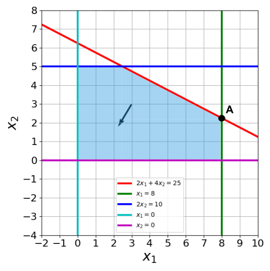
The feasible region is shaded in blue, and the vector within it is the cost vector.
At the root of this problem, we solve the relaxed problem with identical objective function and constraints, except for the integer constraints on \(x_1, x_2\). The LP solution we get is point A on the above graph, \((8, 2.25)\), with an objective value of -35.25. We push this to the priority queue.
As the solution \((8, 2.25)\) is not integer-valued, we need to branch by adding constraints \(x_2 \le 2\) and \(x_2 \ge 3\). Since we know that we must have an integer solution, these constraints remove all non-integer solutions between 2 and 3, while remaining in the inequality format. This creates 2 subproblems, shaded below in green and red. The solutions to these subproblems have costs -34 and -34.5 respectively, so we explore (pop off from the priority queue) red first.
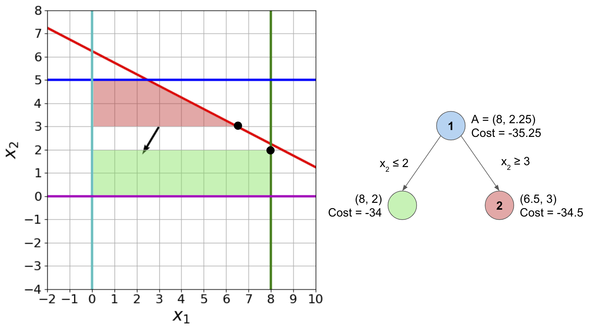
Subproblem 2: solution is (6.5, 3), with cost -34.5. We need to keep branching, because this solution is not integer-valued.
Try walking through the rest of the branch and bound algorithm yourself.
The final search tree with the subproblem and solution at each node is shown below. The nodes are numbered in the order we explore them, i.e., pop them from the priority queue.
Note: the search tree below includes only explored LP solutions.
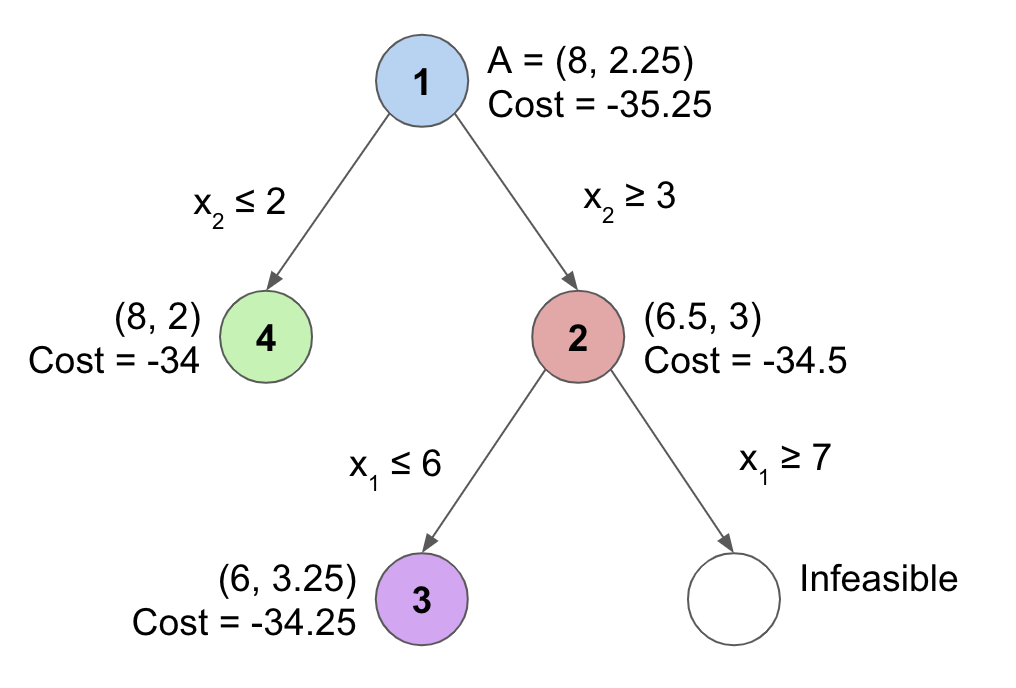
The IP solution returned in the end is (8, 2), with cost -34. A full walkthrough in slide deck format can be found here.
For each of the tree leaves, try to identify the reason we bounded the tree, i.e., why we didn't search further.
For this IP, could a different priority be used to explore the optimal IP solution faster?