We would like to use state space design techniques to design the controller and any filter. We want to identify a state vector, an action vector, and A, B, C, and D matrices for a discrete time system with some sampling rate. After choosing a state vector and an action vector, there are two main ways to estimate the A, B, C, and D matrices.
We don't have information about the individual components described above, although one might for a robot with more expensive components. We will do a lumped model that has free parameters for the effects described above.
Units: Let's use radians for wheel angle. The command has no known units, so we should just use it as is.
Since angular_velocity and current are not measured, they have to be estimated in order to use the direct regression modeling approach. It is easy to estimate velocity as the low pass filtered differences of angles (difference(k) = (angle(k+1)-angle(k-1))/2T where T is the sampling period). Motor current can be generated by guessing a first order low pass filter time constant and low pass filtering the input command signal. One would try to fit models with different time constants to find the appropriate time constant.
We can add past measurements and commands to the state vector to handle the above dynamics, delay, and more complex dynamics. We could include any of angle(k), angle(k-1), angle(k-2), ... and torque(k), torque(k-1), torque(k-2), ... This boils down to ARMA modeling. This approach avoids the need of estimating missing state vector components like velocity or current.
The
frequency-response-based approach only requires measurement of the input
and output of the system.
This page describes how to collect a
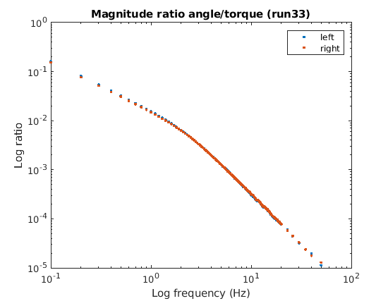
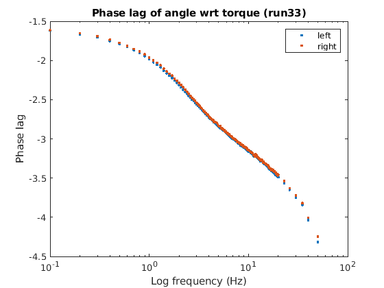
frequency response. The Bode plots for the motor command to wheel angle
are shown below.
There is good agreement between the left and right sides.


I will show how to fit the simplest model (state x = (angle, angular_velocity), action u is the motor_command) to the frequency responses above. I will leave it to you to fit more complex models.
I will first define some constants (some of which I will just guess values for).
Ts = 0.002;
c0 = 0.02;
c1 = 0.004;
Ts is the sampling period (2 milliseconds). c0 and c1 are coefficients in this dynamics equation:
angular_velocity_next = angular_velocity - c0*angular_velocity + c1*motor_command
I will define the various matrices, using my knowledge of the form of the dynamics.
A = [ 1 Ts
      0 1-c0 ]

B = [ 0
      c1 ]

C = [ 1 0 ]

D = [ 0 ]
The first row of A transforms the angular velocity into the position with
Euler integration:
angle_next = angle + Ts*angular_velocityI am assuming this equation is correct. The second row of A and B reflect the following dynamics equation:
angular_velocity_next = angular_velocity - c0*angular_velocity + c1*motor_commandI am assuming that angle has no effect on angular_velocity_next.
One could simulate this system at different frequencies and build a frequency response curve. Matlab provides a way to do this in a few steps: After typing
load fff33.matto load the actual frequency response to compare to, one can type the following to show the comparison.
sys = ss( A, B, C, D, Ts )

w = logspace(-1,1.7,50)

H = freqresp( sys, w, 'Hz' );

figure(1)
hold off
loglog( w, abs( reshape( H(:,:,:), 1, [] ) ) )
hold on
loglog( fff33(:,1), fff33(:,2) )
legend('model','reality')
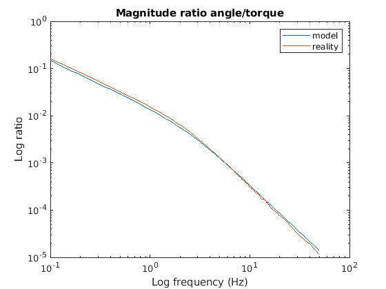
title( "Magnitude ratio angle/torque" )
xlabel( "Log frequency (Hz)" )
ylabel( "Log ratio" )

figure(2)
a = angle( reshape( H(:,:,:), 1, [] ) );
for i = 1:length(a)
  if a(i) > 0
    a(i) = a(i) - 2*pi;
  end
end
hold off
semilogx( w, a )
hold on
loglog( fff33(:,1), -fff33(:,3) )
legend('model','reality')
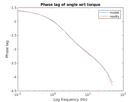
title( "Phase lag of angle wrt torque" )
xlabel( "Log frequency (Hz)" )
ylabel( "Phase lag" )
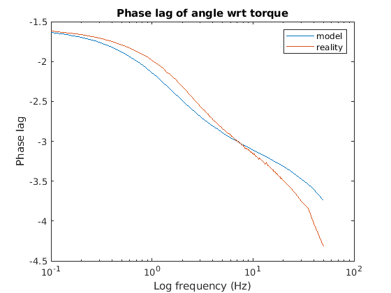
This results in the following Bode plots: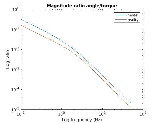
By adjusting c0 and c1, either manually or using the Matlab optimization
routines, you can get the fits below.
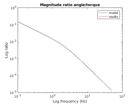
The model magnitude is below reality
at low frequencies and above reality at high frequencies. This is potentially
due to the effect of the declining battery
voltage during the data collection.
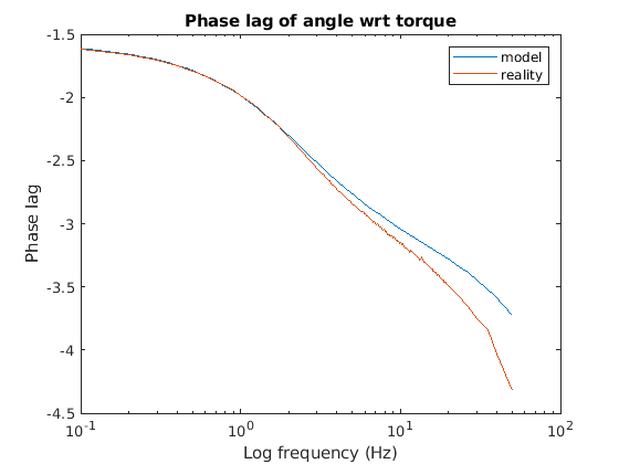
The phase error suggests we need
to add variables to the state vector to increase the phase lag (delay) of
the model at higher frequencies. Pure delay does not affect the
magnitude plot, which already fits well.
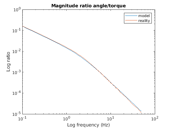
The following plots show an attempt to use direct regression to estimate
the coefficients of the model.
In this case
the velocity had to be estimated, using a combination of differencing
and low pass filtering.
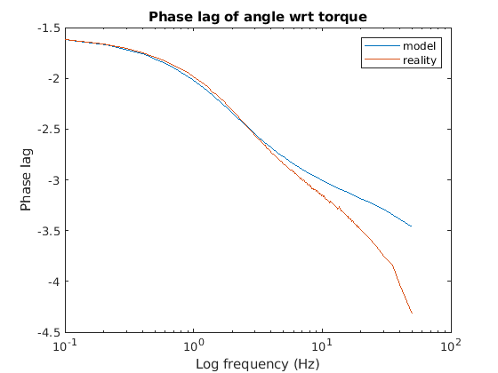
Again, the phase error suggests we need to add variables to the state vector to increase the phase lag (delay) of the model at higher frequencies.
By adding delay variables to the state vector you can get this fit:
model-steps.zip includes versions of parse-data.c and create-commands.c appropriate for the servo output format, and an alternative to process.m, regress_left.m, that sets up the data for a regression to estimate the coefficients of a model. Look at the file model-steps/notes.txt.