I decided to implement the potential function described in class. I did this because it was clearly well-reasoned (and historically frequently used), while previous tinkering with potential functions on my own had not generated the best results.

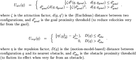
This function is comprised of two componenents summed together, an attractive potential and a repulsive potential. These are given by:

And their gradients, which can be followed to a local minima, are given by:

I reused the map description file format from the previous two assignments but this time reworked the user interface to use FLTK as I had approached the limits of what GLUT could reasonably do.

Like last time, I used a discrete/rasterized grid because it was clear that some interesting implementational details would arise that wouldn't were I working with idealized geometry. In order to compute the potential field, several passes are performed. First, a grid of distances to the goal is filled in by computing the Euclidean distance from the goal to each point. Then, a brushfire/wavefront-style algorithm is executed to compute the 8-point-connectivity distance from each point to the nearest obstacle. This is performed by initializing all cells adjacent to an obstacle to distance 1 and then growing from there. Finally, a pass is performed computing a potential for each cell whose value is given by the equations above.

To follow a path in the potential field, I simulate starting at the start position and following the downward gradient of the field by moving to an adjacent cell of lower potential. This will bring us to a local minima, which is hopefully but not necessarily the goal.

After some tweaking, I settled on 3, 10000, 7.5, and 10 as the attractive factor, repulsive factor, goal threshold, and obstacle threshold, respectively. I settled on these simply because they seemed to work well.

Shown below are several examples of the algorithm's execution.

Successful run
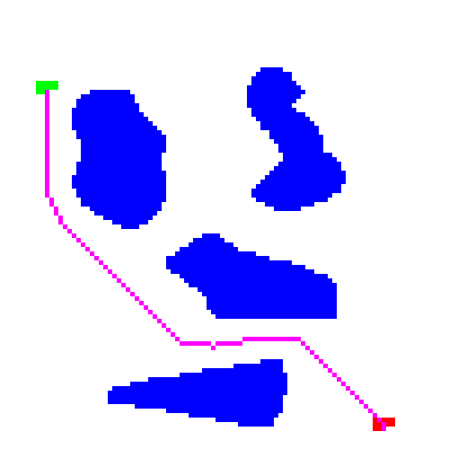
In this example, the planner is able to successfully navigate around an obstacle field.
Path taken:

Distance-to-goal field:

Distance-to-obstacle field:

Total potential field (low dynamic range):

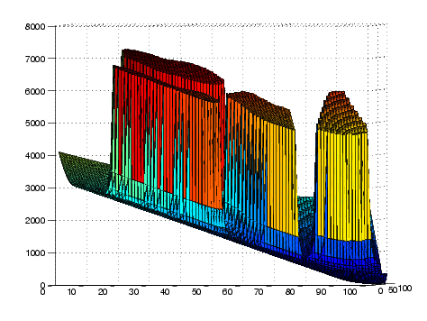
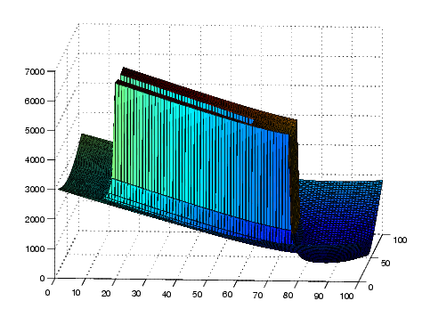
Total potential field (3d surface):

Unsuccessful run
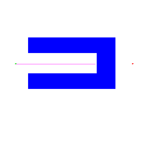
In this example, the planner fails to reach the goal because it falls into the classic horseshoe local minima.
Path taken:

Distance-to-goal field:

Distance-to-obstacle field:

Total potential field (low dynamic range):

Total potential field (3d surface):

Source code: Available here
Videos: Available here

This appears to compile and run fine on linux.andrew.cmu.edu, and should do the same on most other Linux systems. No attempt was made to target other OSes.