1. Implement a PRM planner for a multi-link (at least four) robot arm.

The PRM variant I implemented for this assignment is the RRT. I chose this over the traditional PRM because RRTs seem to be what's used in practice lately and are something that I wanted more experience with. This proved to be a fruitful experience because though the algorithm is remarkably simple, there are subtleties to making it work well.

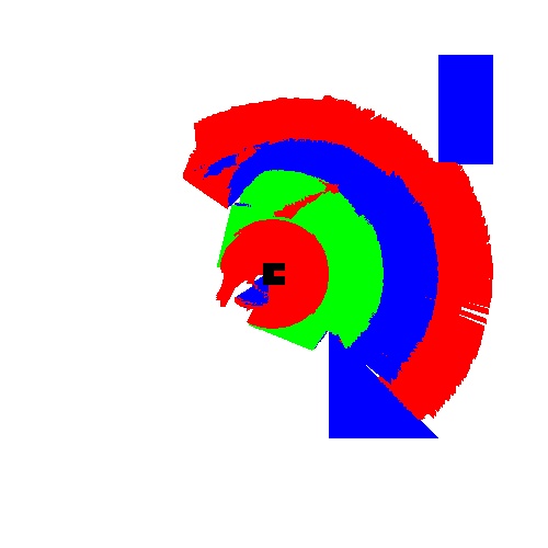
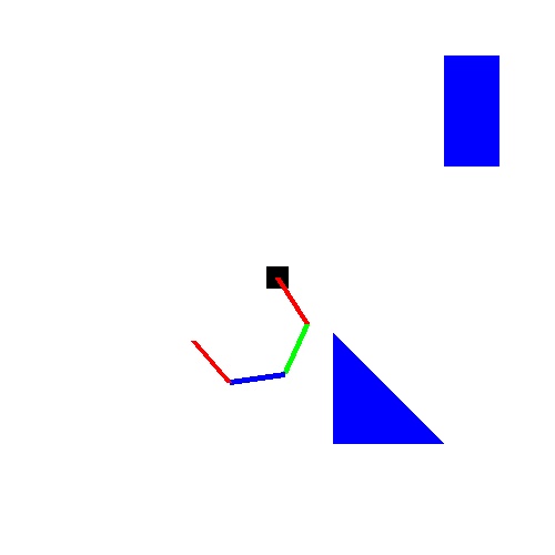
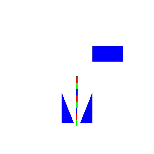
I implemented the RRT planner for a multi-link arm in 2-D. Below are examples for a 4-link and 8-link arm. The world is centered at the fixed base of the arm and includes arbitrary polygonal obstacles.

The algorithm proceeds roughly as follows:

1. Create an explicit search tree comprised of the singleton start state.
2. While !s.isReachable(goalstate) for all s in tree:
   1. s_rand = generate_random_config
   2. s_nearest = find_nearest(s_rand)
   3. if (s_new = expand_tree(s_nearest, s_rand)) != NULL:
      1. add_child(s_nearest, s_new)

Component explanation:

1. States. A state is comprised of a robot configuration, in the form of a tuple of joint angles, one for each joint of the arm.
2. s1.isReachable(s2). This is a function that returns true iff s2 can be reached from s1 by merely linearly interpolating the joint angles between each without any part of the arm intersecting an obstacle along the way. This test is performed by sampling the line of configurations between the two at a resolution that is adapted to be proportional to the speed of the end-effector during the trajectory.
3. generate_random_config. This function returns a robot configuration with joint angles each independently uniformly sampled from (-Pi,Pi]. A goal bias is introduced here so that 20% of the time, the goal state is returned instead of an actual random configuration. This is to bias the search towards the location of the goal.
4. find_nearest(s). This function returns the node in the search tree ``nearest'' the state s. I experimented with two metrics for this purpose: euclidean distance between end-effector positions (orientation disregarded) and sum-of-squares difference (around the unit circle) in the joint angle vectors. Both appeared to work about as well as the other. For this assignment, I implemented this naively by exhaustively comparing against every node in the existing tree. This slowed the planner significantly and should be replaced by a fancier data structure such as a KD tree.
5. expand_tree(s1, s2). This function attempts to expand the search tree by returning a new state that lies on the linear spline between s1 (a node already in the search tree) and s2 (a node outside the search tree). This is performed by progressively sampling along this line (again with adaptive resolution) and stopping when either an obstacle is hit or s2 is reached. The state at that point is returned.
6. add_child(s1, s2). This function inserts s2 into the search tree -- of which s1 is already a member -- as a child of s1.

Examples

Initial configuration:

Configurations searched:

Final configuration:

Initial configuration:

Configurations searched:

Final configuration:

Videos: Available here

Source code: Available here

This appears to compile and run fine on linux.andrew.cmu.edu, and should do the same on most other Linux systems. No attempt was made to target other OSes.