Quantitative Evaluation

Tracker prediction error v.s. prediction time horizon.

As we use the current motion estimate to predict the track position into the future, we expect that the quality of the match beween the prediction and the actual measurement will degrade. This does not directly evaluate the accuracy of the of the track motion estimation, but rather the combined effect of estimation inaccuracy and any failing of the constant-acceleration constant-turn-rate model to capture the actual time-varying behavior of the tracked object.

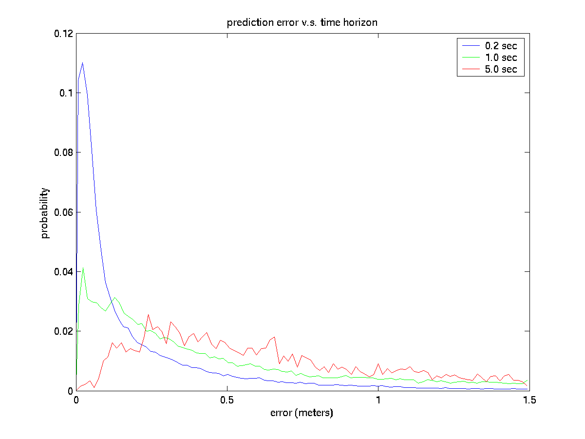
To do this measurement, we use the linear features extracted from the raw scan at the future time and find the RMS distance between the predicted feature position and the measured one. Unfortunately, over the longer time horizons the features may not correspond that well. The tracker itself has considerable internal mechanism to suppress the effects of bad feature correspondences, but this simple validation procedure does not. Hence I believe that the large prediction errors are probably more due to a failure of this validation procedure, rather than actual prediction error.

Be that as it may, in this next plot, we can see the expected pattern where prediction error degrades with time horizon. This plot suggests that prediction is good at 1 second, but dicey at 5 seconds. As noted above, true preformance may be somewhat better, but this does roughly correspond with other estimations that e.g. Christoph has done of vehicle motion predictability.
(Same image in embedded postscript format)

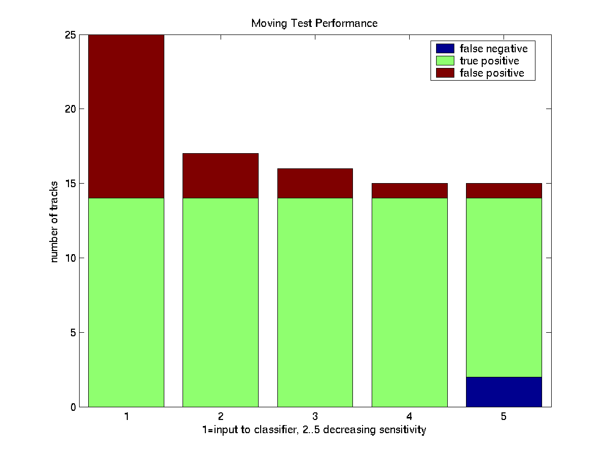
Performance of History-Based Moving Test

In addition to the basic recursive KF tracker structure, there is also a post-pass track validation step which is used to assess our confidence that a track is really moving. This tests how well the current motion estimate can backward-predict the recent past measurements (back about 1/3 second.) If we have solid returns on an object which is in fact rigid and our motion estimate is accurate, then we should get good feature correspondence. If we don't, then something is wrong. Either the object is noisy, or non-rigid (ground return, foliage), we have missing returns, or the object has rapidly changing motion.

Subjectively, this test seemed quite effective in reducing false positive motion reports. To evaluate this, I looked at a minute of data with numerous people and vehicles in it. I then looked at all of the tracks that were identified as moving prior to the history-based moving test and classified them as truly moving if they corresponded to a car or person that appeared to be moving, and false positive if they corresponded to some other object. This is classification is shown in bar 1.

I then turned on the moving test, using several different sets of sensitivity parameters. In condition 2 we are most willing to believe that tracks are moving, in 5 least willing. The blue or "false negative" are tracks that were correctly identified as moving at higher sensitivity settings, but at the lowest sensitivity are marked non-moving.

In this graph, clearly the incidence of false positive motion reports is greatly reduced, and at moderate parameter settings good results can be acheived with minimal increase in false negatives.

This evaluation procedure does not measure all false negatives, only those that introduced by the history-based moving test. The history motion test is only applied to tracks that have:

Mahalanobis distance of velocity estimate from zero > 6 sigmas
Magnitude of velocity estimate > 0.75 meters/sec.

(Same image in embedded postscript format)