Bayesian Color Constancy

In machine vision and image database applications color is often used as a simple means of segmenting or identifying a specific object. Although color in and of itself is often insufficient to perform such a task reliably it can be used robustly in conjunction with other features or as a means of identifying likely candidate regions. When used to identify likely candidate regions, it can speed up the recognition process immensely as described in Rowley (1998). This works well when all of the images are captured with a single camera and under uniform illumination conditions. Problems arise when capture conditions change. The problem is that the measured red, green, and blue (RGB) pixel values are a function of the original object surface reflectance properties, the properties of the illuminant incident on the object surface, and the properties of the camera sensors.

The goal of color constancy is to recover the original surface reflectance properties, S(x,y), regardless of the incident illumination. It has been shown in Finlayson (1993) that with a relatively mild set of assumptions, illumination effects (under some canonical camera model) can be collapsed to the following simple form, where the measured pixels values for channel k at location (x,y) are denoted as $\rho _{k}(x,y)$ :

$R=\rho _{r}(x,y)=\alpha S_{r}(x,y)$ ; $G=\rho _{g}(x,y)=\beta S_{g}(x,y)$ ; $B=\rho _{b}(x,y)=\gamma S_{b}(x,y)$

In this form all that needs to be estimated are the three values $\alpha$ , $\beta$ , and $\gamma$ in order to recover surface reflectance information and compute a color feature value which is invariant of incident illumination.

Impact:

Color constancy is not only important for machine vision applications but is also important for digital cameras and scanners. Frequently images are captured under varying lighting conditions. This can lead to images having an reddish tone if captured under tungsten illumination or a greenish tone if captured under fluorescent lighting. Color constancy can be used as a means of removing those color casts resulting in a more visually pleasing image.

State of the Art:

Many color constancy methods are described in the literature: Land (1977), Finlayson (1995), Funt (1996), Brainard (1997). These methods estimate illumination parameters by making a set of prior assumptions about the overall distribution of color values in a typical image, or correspondingly, typical illuminants and surfaces in the world.

One algorithm, described in Finlayson (1995), utilizes constraints about the colors of typical object surfaces and illuminants in the world and applies them to the distribution of the extreme colors in an image. A search procedure is used to determine the transformation which best satisfies the given constraints.

A method introduced in Funt (1996) uses a neural network which takes as input the image color histogram and outputs the estimated illuminant chromaticities.

Approach:

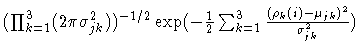
This work attempts to overcome some of the deficiencies of more basic algorithms through the construction of a parametric model of the distribution of color channel responses in an image and the use of that model as the basis for computation in lieu of the raw pixel values. The parametric model chosen is a mixture of Gaussians. In this model every three dimensional pixel value (R,G,B) is modeled as being generated by one of the model Gaussians with a hidden indicator variable, z_ij, representing which Gaussian generated which pixel. In the equations below we index the pixels in the image by the variable i, ranging from 1 to m where m is the number of pixels in the image, the other variables are defined as follows: the variable j indexes the n Gaussians in the mixture and the variable k indexes the color channels (dimensions), ranging from 1 to 3:

$Pr(\rho _{r}(i),\rho _{g}(i),\rho _{b}(i)\mid z_{ij},\mu ,\sigma )\: \sim$ $(\prod _{k=1}^{3}(2\pi \sigma _{jk}^{2}))^{-1/2}\exp ( -\frac{1}{2}\sum _{k=1}^{3}\frac{(\rho _{k}(i)-\mu _{jk})^{2}}{\sigma _{jk}^{2}})$

To build the model, we must estimate the Gaussian parameters as well as the expected values of the indicator variables. As is typically done, as per Duda (1973), we use Expectation-Maximization (EM) to estimate these parameter values. A computationally efficient procedure is described in Moore (1999).

Once the components of the mixture model have been identified, a maximum likelihood approach can be used to determine the illumination parameters which maximize the likelihood of the observed data. In a manner similar to Brainard (1997), we assume that the likelihood of a specific setting of the illumination parameters, I_j, given the observed cluster centers, ${\bf V}$ , can be factored as follows:

Note that the value of the corrected color S_i can be determined simply from ${\bf V}$ because of the multiplicative effect of the incident illumination.

Future Work:

There are a number of possible future directions to take in this work. One is to try to relax the independence assumption. Another is to try use some other criterion like BIC as a means of choosing the number of mixtures in the mixture model.

**Figure 1:** An example of two raw images: (a) captured under halogen illumination and (c) captured under fluorescent illumination. Their respective versions normalized for illumination color, (b) and (d), were processed by an early version of our EM based algorithm. If these images do not appear in color, they can be found online at: http://www.cs.cmu.edu/~chuck/cc1/
$\begin{figure} \par\begin{center} \begin{tabular}{cccc} \epsfig{file=cruncheroo... ...{center}\par\vspace{-0.10in}\parskip +0pt\rule{\textwidth}{.2mm} \end{figure}$

Bayesian Color Constancy

Problem:

Impact:

State of the Art:

Approach:

Future Work:

Bibliography

About this document...