[3 points] Recall that, one way to represent the nodes of a complete binary tree is with a list, where the first element contains the root, the next two elements contain the next level of the tree (the children of the root), the next four elements contain the next level of the tree (two containing the children of the root's left child and then two containing the children of the root's right child), the next eight elements contain the next level contains (two children of each of the nodes at the previous level), and so on, depending on how many levels the tree has.

The binary tree at left with nodes labeled "a" through "o" would be represented by the Python list:
   ["a","b","c","d","e","f","g","h","i","j","k","l","m","n","o"]
     0   1   2   3   4   5   6   7   8   9  10  11  12  13  14

This representation can be extended to incomplete trees by using None to represent the "missing" nodes that would need to be added to make a complete tree. This is the case for the tree to the left, which can be represented by the Python list:
["a","b","c","d","e",None,"g","h","i",None,"k",None,None,"n","o"]
Observe that:
-
The left child of the node at index 0 (labeled "a")
is the node at 1 (labeled "b").
The left child of the node at 1 ("b") is the node at 3 ("d").
The left child of the node at 2 ("c") is the node at 5 ("f").
The left child of the node at 3 ("d") is the node at 7 ("h").
The left child of the node at 4 ("e") is the node at 9 ("j").
The right child of the node at 2 ("c") is the node at 6 ("g").
The right child of the node at 3 ("d") is the node at 8 ("i").
The right child of the node at 4 ("e") is the node at 10 ("k").
The parent of the nodes at 3 ("d") and at 4 ("e") is at 1 ("b").
The parent of the nodes at 5 ("f") and at 6 ("g") is at 2 ("c").
The parent of the nodes at 7 ("h") and at 8 ("i") is at 3 ("d").
Do you see a pattern? There are simple formulas that can be used to calculate the indices of a node's left child, right child, and parent from that node's index.
Define a function left_index(index) (in left_index.py) that, when passed the index of a node, will return the index of that node's left child. (You do not need to worry about whether the node has a left child; when the node does not actually have a left child, the function should still return where its left child would be if it had one. You may assume that index is a non-negative integer.)
Define a function right_index(index) (in
right_index.py) that, when passed the index of a node,
will return the index of that node's right child.
(You do not need to worry about whether the node has a right
child; when the node does not actually have a right child, the
function should still return where its right child would
be if it had one. You may assume that
Define a function parent_index(index) (in parent_index.py) that, when passed the index of a node, will return the index of that node's parent. (You may assume that the index is a positive integer.)
[2 points] The ancestors of a node in a tree are defined to include the node itself, the parent of that node, the parent of the parent, the parent of the parent of the parent, etc., up to and including the root of the node.
The following algorithm prints out the labels of the ancestors of the node at index i in the list tree, which is a list representation of a complete binary tree as described above.
-
Print out the label of the node at index i in tree
with a new line.
If i is not the index of the root, then do the following:
-
Set j equal to the index of the parent of the node
at index i in tree.
Recursively, print out the ancestors of the node at index
j of tree.
In ancestors.py, using the algorithm above define a function ancestors(tree,i), which requires a list tree encoding a binary tree as described above and an index i of a node in the binary tree. When called, ancestors(tree,i) should print out the labels of the ancestors of the node at index i starting with the node at i and going through the root of the tree. Note that the algorithm is recursive. Your solution must also be recursive, as specified.
You should call your parent_index function from problem 1 to compute the value for j in the algorithm above. This means you should have a copy of the parent_index function in your ancestors.py file, at the top of the file before you define the function for ancestors.
You may assume that tree is complete, i is a non-negative index less than the length of tree, and that tree[i] is not None.
Example:
> python3 -i ancestors.py
>>> tree = ["a","b","c","d","e","f","g","h","i","j","k","l","m","n","o"]
>>> tree
["a", "b", "c", "d", "e", "f", "g", "h", "i", "j", "k", "l", "m", "n", "o"]
>>> ancestors(tree,8)
i
d
b
a
>>> ancestors(tree,5)
f
c
a
>>> ancestors(tree,0)
a
[2 points] In a Binary Search Tree, each node has a value that is greater than that of all of the nodes reachable through its left child and that is less than that of all of the nodes reachable through its right child. (We will assume that the tree does not hold two nodes with the same value.) A Binary Search Tree can be stored using a list just as we did in the previous problems.
The following is an algorithm for searching a list called tree encoding a binary search tree to determine whether it contains a node with the value key.
-
Set curr_index to the index of the root node of the tree.
While curr_index is valid and the value of the
node at curr_index is not None,
do the following:
-
Set curr_value to the value of the node at
curr_index in tree.
Return True if curr_value is equal to key.
Set curr_index to the index of the left child
of the node at curr_index if key is less than
curr_value.
Set curr_index to the index of the right child
of the node at curr_index if key is greater than
curr_value.
Define a function bst_search(bst,key) (in bst_search.py) that uses this algorithm to determine whether the value key occurs in bst, the list representing a binary search tree.
Call the functions left_index and right_index that you defined in problem 1 to set curr_index in substeps C and D above. This means you should have a copy of the left_index and right_index functions in your bst_search.py file, at the top of the file before you define the function for bst_search.
Example:
> python3 -i bst_search.py
>>> bstree = [84, 41, 96, 25, 50, None, 98]
>>> bstree
[84, 41, 96, 25, 50, None, 98]
>>> bst_search(bstree, 50)
True
>>> bst_search(bstree, 51)
False
>>> bst_search(bstree, 41)
True
>>> bst_search(bstree, 90)
False
Recall that a graph of \(n\) nodes can be represented as an \(n \times n\) matrix where the value at row \(i\) column \(j\) gives the "cost" of going directly from node \(i\) to node \(j\) in the graph.
The following \(O(n^3)\) algorithm computes the lowest cost (shortest) path from each node in the graph to a given destination node \(d\):
-
Set \(n\) equal to the number of nodes in the graph.
Set best_cost_to_d equal to a new list with \(n\) elements.
For \(i\) in the range 0 to \(n-1\) inclusive, do the following:
- Return the best_cost_to_d list, which will now contain the minimum cost to to \(d\) from each location.
-
Set best_cost_to_d[\(i\)] equal to the cost of going directly from
node \(i\) to node \(d\).
-
For \(i\) in the range 0 to \(n-1\) inclusive, do the following:
-
For \(j\) in the range 0 to \(n-1\ inclusive), do the following:
-
Let cost_from_i_to_j be the cost of going
directly from node \(i\) to node \(j\) in the graph.
Let cost_from_i_to_d_via_j be
cost_from_i_to_j + best_cost_to_d[\(j\)].
If cost_from_i_to d_via_j is less than
best_cost_to_d[\(i\)] then it's cheaper to
go to d via node j, so
set best_cost_to_d[\(i\)] to
cost_from_i_to_d_via_j.
Write the following two functions:
[2 points] Write a function shortest_path(graph,d) (in shortest_path.py) that takes graph (a two-dimensional list holding the costs of traversing the graph's edges as described above) and d (the index of the destination node) and returns an list with the costs of the shortest path to node d from each node in the graph, using the algorithm above as your guide.
Example usage:
> python3 -i shortest_path.py
>>> f = float("inf")
>>> graph1 = [[0,4,5,6,2],[4,0,10,3,1],[5,10,0,7,9],[6,3,7,0,8],[2,1,9,8,0]]
>>> graph1
[[0,4,5,6,2],[4,0,10,3,1],[5,10,0,7,9],[6,3,7,0,8],[2,1,9,8,0]]
>>> shortest_path(graph1, 0)
[0, 3, 5, 6, 2]
>>> shortest_path(graph1, 3)
[6, 3, 7, 0, 4]
>>> graph2 = [[0, 6, 7, 5],[2, 0, 4, f],[2, f, 0, 3],[f, f, 9, 0]]
>>> graph2
[[0, 6, 7, 5],[2, 0, 4, inf],[2, inf, 0, 3],[inf, inf, 9, 0]]
>>> shortest_path(graph2, 3)
[5, 7, 3, 0]
In the first example, shortest_path(graph1, 0) give the cost of the shortest path in the first graph from node 0 to all of the other nodes. Note that the cost of the shortest path from node 0 to itself is 0 since you're there already.Also note that in the graphs, the cost of going from a node to itself is 0, but the cost from going to a node to another node that is not connected to it is infinity.
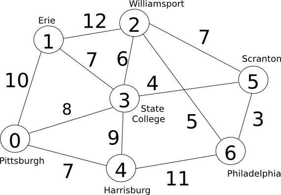
[1 point] Write a function test_sp() (also in shortest_path.py) to test your shortest path algorithm. The function should create a 2D matrix for the graph below and then call your shortest_path function with a destination of node 0, returning its answer.
Example usage:
>python3 -i shortest.path.py
>>> test_sp()
[0, 10, 14, 8, 7, 12, 15]
Looking at the results in this case, it says that the shortest paths to Pittsburgh from all cities are as follows:
From node:            Cost of shortest path:
0 (Pittsburgh)        0  (already there)
1 (Erie)              10 (direct)
2 (Williamsport)      14 (through State College)
3 (State College)     8  (direct)
4 (Harrisburg)        7  (direct)
5 (Scranton)          12 (through State College)
6 (Philadelphia)      15 (through State College and Scranton)
Try out other destinations to see what you get.
Submission
You should now have a pa6 directory, containing:
-
left_index.py
right_index.py
parent_index.py
ancestors.py (also containing the function parent_index)
bst_search.py (also containing the functions left_index and right_index)
shortest_path.py (containing the functions shortest_path and test_sp)
Zip up your directory and upload it using the autolab system.