def f(n):
    if n % 3 == 0 or n < 3:
        return n * (n - 1)
    else:
        return f(n // 2) + f(n - 2)
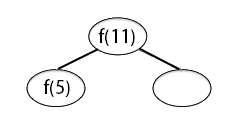
Trace the computation of f(11) by drawing a recursion tree (like the one for Fibonacci numbers on the slides for Lecture 9), showing all of the recursive calls that need to be computed to find the value for f(11). Then using your recursion tree, compute the value of f(11). We've started the tree for you below:

[2 points] This question is about simple recursions on lists. We saw in class that a standard way of splitting a list items is into its "head", using items[0], and its "tail", using items[1:]
- In general, if a is a list of numbers, what does
g(a) return?
def g(a): if a == []: return 0 else: return a[0] + g(a[1:]) - We can split a list up in other ways, too.
In Python, you can use negative
index values when accessing list elements. These count backwards
from the end of a list with -1 being an index for the last element in
an array. The range notation for "slicing" lists can also use
negative elements or a mix of positive and negative elements.
For example:
>>> a = ['v', 'w', 'x', 'y', 'z']
>>> a[-1]
'z'
>>> a[-2]
'y'
>>> a[-3]
'x'
>>> a[-3:]
['x', 'y', 'z']
>>> a[-3,-1]
['x','y']
>>> a[:-1]
['v','w', 'x','y']
Consider the following Python function. Given a list of numbers
a, what doesh(a)return? You may find it useful to trace what it does for a particular input.def h(a): if a == []: return 0 else: return a[-1] + h(a[:-1])
- [2 points] Do you believe that the recursive binary search algorithm we
saw in class works in all cases? What about "edge cases", such as a key that
precedes the first element in the list or follows the last element?
What if the integer division (lower + upper) // 2 causes
problems when the list has an even number of elements? For this
problem you will investigate this question. To help you, here is the
Python code from lecture:
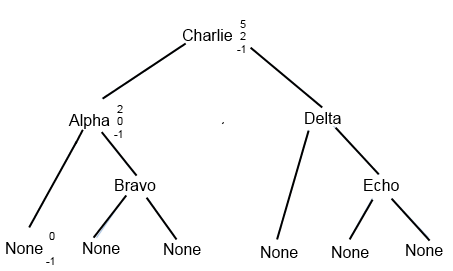
One way to convince yourself that the algorithm works is to show that every possible position in the ordered list, including both the values themselves (when the key is found) and the positions between values (when the key is not found and the binary search should return None), can be derived by following the algorithm for updating mid, lower, and upper. To do this, we're going to construct a complete binary search tree. First we introduce some notation for depicting nodes in the search tree. Each node corresponds either to a value in the list being searched, or to a base case where the search would fail. The X on the left below illustrates the first case, and the None on the right below illustrates the second case:# main function def bsearch(items, key): return bs_helper(items, key, -1, len(items)) # recursive helper function def bs_helper(items, key, lower, upper): if lower + 1 == upper: # Base case: empty return None mid = (lower + upper) // 2 # Recursive case if key == items[mid]: return mid if key < items[mid]: # Go left return bs_helper(items, key, lower, mid) else: # Go right return bs_helper(items, key, mid, upper)X upper mid lower None upper lower We have started the binary search tree diagram below. You will complete it by filling in the numbers as appropriate for each node, showing that every node can be reached by the search function, and proving that if a key is in the list, the algorithm will find it.
In the diagram below, we've filled in the numeric values for three of the nodes for the case where the key is "Aardvark". The binary search always begins with lower = -1 and upper = 5, giving mid = 2, which puts us at "Charlie". So all searches of this list start at "Charlie". If the key is less than this value, the algorithm tells us to set upper equal to mid, so we have upper = 2 and lower = -1, which gives mid = 0, taking us to node "Alpha", as shown. If we go left from "Alpha" (because the key is less than "Alpha"), the next node has upper = 0 and lower = -1. Since now lower+1 = upper, the algorithm returns None, making this node a terminal (leaf) node. Print out the diagram, or redraw it yourself, and complete the tree by following the algorithm to fill in all the missing values, so that every node has either two or three numbers written next to it. For example, you might choose a key of "Bravo" and see how the algorithm gets to that node. Then choose a key of "Banana" and see at which leaf node the algorithm ends. And so on. Include your complete annotated tree in the pages you hand in.
items = ["Alpha", "Bravo", "Charlie", "Delta", "Echo"]
- [1 point] Suppose that you have a "budget" of 5 key comparisons for searching for a key in a sorted list. That is, your search would terminate after comparing the key to at most 5 list elements. With this budget, what is the size of the largest sorted list that you could search using binary search? (Note: "key comparison" refers only to comparisons involving the key being searched for.)
Show how the merge step would behave by completing the trace below. Add a line to the trace for each element that is placed in the output, crossing the element off the input as shown.
| First half | Second half | Output list |
| 4, 18, 20, 55, 87, 90 | 1, 25, 27, 44, 88 | |
| 4, 18, 20, 55, 87, 90 | |
1 |
For example, if we want to sort the list
list = [56, 42, 82, 75, 18, 58, 27, 61, 84, 41, 21, 15, 71, 90, 33]we create two lists, separating the elements based on the pivot 56:
list1 = [42, 18, 27, 41, 21, 15, 33]
list2 = [82, 75, 58, 61, 84, 71, 90]
Each sublist is sorted recursively (final results shown for each sublist):
list1 = [15, 18, 21, 27, 33, 41, 42]
list2 = [58, 61, 71, 75, 82, 84, 90]
and the final result is
[15, 18, 21, 27, 33, 41, 42] + [56] + [58, 61, 71, 75, 82, 84, 90]
=> [15, 18, 21, 27, 33, 41, 42, 56, 58, 61, 71, 75, 82, 84, 90]
Suppose we apply Quicksort to the list
[47, 55, 50, 20, 18, 47, 17, 25, 17]. Show the two (unsorted) sublists that result from splitting based on the pivot.For the best performance of Quicksort, would we rather have the two sublists of equal length, or would we rather have one be very short and the other very long? Explain briefly.