Local Search
Learning Objectives
Describe and implement the following local search algorithms:
Iterative improvement algorithm with min-conflict heuristic for CSPs
Hill Climbing (Greedy Local Search)
Random Walk
Simulated Annealing
Identify optimality of local search algorithms
Compare different local search algorithms as well as contrast with classical search algorithms
Select appropriate local search algorithms for real-world problems
Characteristics and Advantages
Local search algorithms operate using a single current node (rather than multiple paths) and generally move only to neighbors of that node.
Two key advantages of local search:
use very little memory (usually a constant amount)
can often find reasonable solutions in large or infinite (continuous) state spaces for which systematic algorithms are unsuitable
Important Learning Goal: As you learn about local searches, try to understand how different local searches relate to each other (specifically, how can you modify one local search to achieve another?)
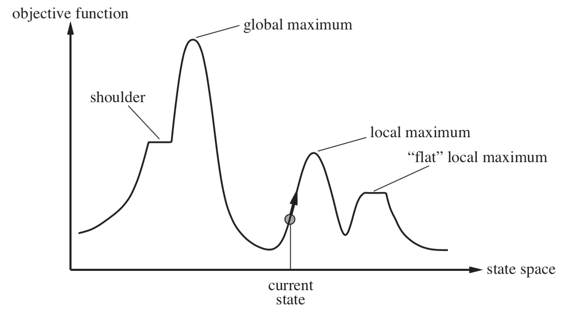
State Space Landscape

Location (x-axis): State
Elevation (y-axis): Heuistic cost function or objective function
Global Minimum: If elevation corresponds to cost, then the aim is to find the lowest valley
Global Maximum: If elevation corresponds to an objective function, then the aim is to find the highest peak
Local Maximum: a peak that is higher than each of its neighboring states but lower than the global maximum
Plateau: a flat area of the state-space landscape (either a flat local maximum, from which no uphill exit exists, or shoulder, from which progress is possible)
Source: AIMA \(4^{th}\) edition, chapter 4, section 1, pages 110-119
Algorithms
Note about Optimality: A local search algorithm is optimal if the algorithm always finds a global maximum/minimum.
Hill Climbing
Motivation: Continually moves "uphill" in state-space landscape, and terminate when it reaches a "peak", or where there is no neighbor with higher value.
def hill_climbing(problem):
    current = node(problem.initialState)
    while True:
        neighbor = Successor of current with highest objective function value
        if neighbor.value <= current.value:
            return current.state
current = neighbor Optimal: No
Variants:
Random-restart Hill Climbing:
Run hill climbing multiple times starting from a random location until the global optima is found.
Stochastic Hill Climbing:
Choose randomly from uphill moves, where probability is dependent on the steepness (how much it increases from current state)
Converges slower than choosing steepest ascent, but may find better solutions
First-choice Hill Climbing:
One implementation of stochastic hill climbing
Generate successors randomly until better one is found
Good to use if there are too many successors
Source: AIMA \(4^{th}\) edition, chapter 4, section 1.1
Random Walk
Uniformly randomly choose a neighbor to move to, and save the best neighbor seen so far. Stop iteration after K moves. As K increases, the solutions returned by random walk should theoretically approach the global optima.
Simulated Annealing
Relation to hill climbing:
Consider a hill-climbing algorithm that never makes "downhill" moves toward states with lower value (or higher cost)
Pro: efficient
Con: it can get stuck on a local maximum
Consider a random walk (moving to a successor chosen uniformly at random from the set of successor)
Pro: It will eventually find a solution
Con: extremely inefficient
Simulated Annealing = HILL CLIMBING + RANDOM WALK
(yields efficiency + ability to find a goal)
How it works
Innermost loop is quite similar to hill climbing
Instead of picking the best move, it picks a random move
If the move improves the situation, the move is always accepted.
Otherwise, it accepts the move with some probability less than 1
The probability of choosing the worse move decreases exponentially
With the "badness" of the move (\(\Delta E\) by which the evaluation is worsened)
As "temperature" T goes down: "bad" moves are more likely to be allowed at the start when T is high, and they become more unlikely as T decreases.
If the schedule lowers T slowly enough, the algorithm will find a global optimum with probability approaching 1
Recall that the probability of choosing a "bad move" is \(\frac{1}{e^{|\Delta E|/T}}\) since \(\Delta E\) is negative for a bad move
Over time, T decreases, so denominator increases
Probability of choosing bad move approaches 0
Probability of not choosing bad move approaches 1
Source: AIMA \(4^{th}\) edition, chapter 4, section 1.2