Search
Learning Objectives
Understand how to formulate and define problems as search problems.
Describe and implement various search algorithms.
Understand how search algorithms run on a given problem.
Analyze the time and space complexity of a variety of search algorithms.
Give example search applications where one search algorithm would outperform others, e.g. a situation where DFS would outperform BFS.
Verify or create admissible/consistent heuristics for a given search problem
Describe the trade-offs between computationally cheap, inaccurate heuristics and computationally expensive heuristics
Understand both the algorithmic differences and the distinct use cases for tree search vs graph search.
Define a game, zero-sum game, standard form, and a game search tree
Trace and implement Minimax, Expectimax, and Expectiminimax given a start state, player list, and actions.
Describe the bounded lookahead algorithm
Define and create evaluation functions
Analyze a minimax tree using alpha-beta pruning to determine pruned nodes
Discuss the ethical implications of a given real-world application involving search algorithms.
Search Agents
An agent is an entity that perceives and acts.
For example, Pacman is an agent that perceives where the ghosts and food are and decides which direction to go in based on that information.
We consider an agent to be rational if the agent maximizes its expected utility.
Rationality depends on:
Performance measure
The prior knowledge that the agent has
The actions available to the agent
What the agent has already perceived and done
Another type of agent is a Reflex agent:
Chooses actions based on current percept
May have intuition about the world's current state
Does not consider the future consequences of their actions
A final type of agent to consider is a Planning agent, which considers how the world would be based on a transitional model and a goal in mind.
Search Problem
A search problem is defined by
State Space
For each state s, a set of allowable actions: Actions(s)
Transition Model: Result(s,a)
Step Cost Function: c(s,a,s')
Start State
Goal Test
A solution to a search problem is defined by the sequence of actions from the start to goal state.
Example
State Space
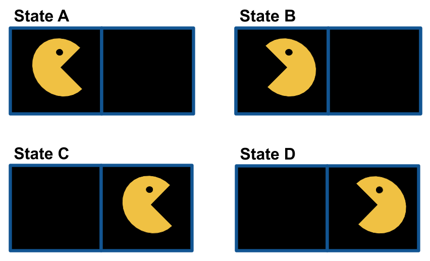
For each state s, a set of allowable actions: Actions(s)
Suppose the agent can rotate 180 degrees clockwise or move forward in the agent's current direction.Actions(A) = {Rotate, Move Forward}
Actions(B) = {Rotate}
Actions(C) = {Rotate}
Actions(D) = {Rotate, Move Forward}Transition Model: Result(s,a)
Result(A, Rotate) = B
Result(A, Move Forward) = C Result(B, Rotate) = A
Result(C, Rotate) = D
Result(D, Rotate) = C
Result(D, Move Forward) = B
Step Cost Function: c(s,a,s')
c(s, Rotate, s') = 1
c(s, Move Forward, s') = 2Start State: A
Goal Test: Is the current state the same as state C?
Search Algorithms
A state space graph is a mathematical representation of a search problem.
Nodes are (abstracted) world configurations
Arcs represent transitions resulting from actions
The goal test is a set of goal nodes
Each state occurs only once
For example, consider the example given for defining a search problem. The corresponding state space graph is below.

We can rarely build this full graph in memory, but it is a useful idea.
Motivation: We can use a search algorithms to find a solution to a search problem. In particular, we can find a path (i.e. sequence of actions) from the start state to the goal state in the state space graph.
Search algorithms can be uninformed search methods or informed search methods.
Tree vs Graph Search
def tree_search(problem):
    initialize frontier as specific work list # (stack, queue, priority queue)
    add initial state of problem to frontier

    while frontier not empty:
        choose a node and remove it from frontier

        if node contains goal state:
            return the corresponding solution

        for each resulting child from node:
            add child to frontier

    return failure
def graph_search(problem):
initialize the explored set to be empty
initialize frontier as specific work list # (stack, queue, priority queue)
add intial state of problem to frontier
while frontier not empty:
choose a node and remove it from frontier
if node contains goal state:
return the corresponding solution
add node to explored set
for each resulting child from node:
if child state not in frontier and child state not in explored set:
add child to the frontier
return failure Based on the pseudo-code for tree search vs. graph search, we can see that the main differences are:
Graph search includes an additional explored set to keep track of nodes we have already visited
When adding new nodes to the frontier, graph search will additionally check that the node has not been previously visited (node is not already in the explored set)

Note that the explored set, the frontier, and never seen have no overlaps (no node is added to a frontier if it has been explored, and once a node is popped off of the frontier, it is added to the explored set)
Graph search detects cycles (able to check if a node has already been visited)
Tree search cannot detect cycles (no way of knowing if a node has already been visited)
Uninformed Search Algorithms
Uninformed search methods have no additional information about the cost from the current node to the goal node.

Examples of uninformed search methods include:
Breadth First Search
Depth First Search
Uniform Cost Search
Iterative Deepening
Breadth First Search
Strategy: expand a shallowest node first
Frontier Data Structure: FIFO Queue
Depth First Search
Strategy: expand a deepest node first
Frontier Data Structure: LIFO Stack
Iterative Deepening
Strategy: repeatedly expand a deepest node first (up to a fixed depth)
Frontier Data Structure: LIFO Stack
combines space efficiency of DFS with completeness of BFS
Note: Breadth first search is complete (meaning it will find a path from the start node to the goal node if it exists). In a graph with equal edge weights, breadth first search can be used to find the shortest path from the start node to the goal node. However, depth first search stores less information in the frontier and is therefore more space efficient.
Example
To see these characteristics in action, consider the following graph:
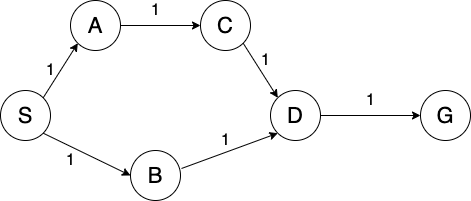
Suppose we run BFS and DFS to find a path from node S to node G (using graph search and breaking ties alphabetically).
BFS
Frontier:
S,S-A,S-B,S-A-C,S-B-D, S-B-D-GExplored Set: S, A, B, C, D
Path: S-B-D-G
DFS
Frontier:
S,S-A, S-B,S-A-C,S-A-C-D, S-A-C-D-GExplored Set: S, A, C, D
Path: S-A-C-D-G
IDS
Limit = 0
Frontier:
SExplored Set: S
Limit = 1
Frontier:
S,S-A,S-BExplored Set: S, A, B
Limit = 2
Frontier:
S,S-A,S-B,S-A-C,S-B-DExplored Set: S, A, C, B, D
Limit = 3
Frontier:
S,S-A,S-B,S-A-C,S-A-C-DExplored Set: S, A, C, D, B
Limit = 4
Frontier:
S,S-A, S-B,S-A-C,S-A-C-D, S-A-C-D-GExplored Set: S, A, C, D
Path: S-A-C-D-G
Path Cost: 10
Notice that BFS returns a shorter path, while DFS has fewer nodes on the frontier. Though DFS found a path to the goal, this is not always the case. We can combine the space-efficiency of DFS with the completeness of BFS. This is the motivation behind iterative deepening.
Uniform Cost Search
Strategy: expand a cheapest node first
Frontier Data Structure: Priority Queue (priority given by cumulative cost)
Note: If we want to find the cheapest path from the start node to the goal node, search algorithms such as BFS and DFS are not guaranteed to give us the right answer. This is where uniform cost search comes in.
Example
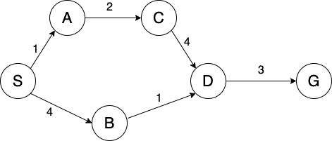
Consider the graph from earlier (now with different edge weights):
BFS
Frontier:
S,S-A,S-B,S-A-C,S-B-D, S-B-D-GExplored Set: S, A, B, C, D
Path: S-B-D-G
Path cost: 8
DFS
Frontier:
S,S-A, S-BS-A-C,S-A-C-D, S-A-C-D-GExplored Set: S, A, C, D
Path: S-A-C-D-G
Path Cost: 10
IDS
Limit = 0
Frontier:
SExplored Set: S
Limit = 1
Frontier:
S,S-A,S-BExplored Set: S, A, B
Limit = 2
Frontier:
S,S-A,S-B,S-A-C,S-B-DExplored Set: S, A, C, B, D
Limit = 3
Frontier:
S,S-A,S-B,S-A-C,S-A-C-DExplored Set: S, A, C, D, B
Limit = 4
Frontier:
S,S-A, S-B,S-A-C,S-A-C-D, S-A-C-D-GExplored Set: S, A, C, D
Path: S-A-C-D-G
Path Cost: 10
UCS
Frontier:
(S, 0),(S-A, 1),(S-B, 4),(S-A-C, 3),(S-A-C-D, 7),(S-B-D, 5), (S-B-D-G, 8)Note: Bolded strike through means node was replaced on the frontier. Specifically,
(S-A-C-D, 7)was replaced by(S-B-D, 5)Explored Set: S, A, C, B, D
Path: S-B-D-G
Path Cost: 8
Informed Search Algorithms

Heuristics
When it comes to informed search, we use something called a heuristic that will estimate how close we are to a goal. The actual function being used to estimate will be designed for the particular search problem.
For each heuristic, we care about two things:
Admissibility: \(0 \leq h(n) \leq h^*(n)\), where \(h^*(n)\) is the true path cost to the nearest goal
Consistency: Estimated heuristic costs \(\leq\) actual costs; If we have a path from A \(\rightarrow\) C then \(h(A)-h(C) \leq cost(A \rightarrow C)\)
Special heuristics:
Zero heuristic: \(h=0\) for all nodes
Exact heuristic: great, but too expensive to compute, or hard to define!
Dominant heuristic: \(h_a\) dominates \(h_c\), i.e., \(h_a \geq h_c\) if \(\forall n,~ h_a(n) \geq h_c(n)\)
Greedy Search
Strategy:expand the node that seems closest to the goal state according to the heuristic \(h\).
Since this is a greedy search, there are a couple of problems with this algorithm:
It will choose a node even if it as at the end of a very long path because the heuristic will see the node as close to the goal
It relies on the heuristic even if the heuristic is wrong
A*
In order to get the benefits of informed search while getting some of the nice properties of uninformed search, we introduce A\(^*\) search.

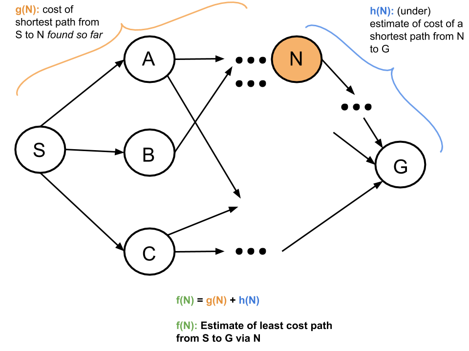
Uniform-cost orders by path cost, or backward cost: g(n)
Greedy orders by goal proximity, or forward cost: h(n)
Combining these two, A\(^*\) Search orders by the sum of the two: f(n) = g(n) + h(n)
Consistency Implies Admissibility
A heuristic is admissible if it never overestimates the true cost to a nearest goal.
A heuristic is consistent if, when going from neighboring nodes \(a\) to \(b\), the heuristic difference/step cost never overestimates the actual step cost.
Let \(h(n)\) be the heuristic value at node \(n\) and \(c(n,n+1)\) be the cost from node \(n\) to \(n+1\). We assume that \(h(g) = 0\). Informally, we want to backtrack from the goal node, showing that if we start with an admissible node (which \(h(g)=0\) is), its parent nodes will be admissible through the rule of consistency, and this pattern continues.
Consider some node \(n\) and assume the heuristic value at \(n\) is admissible. We want to show that any of its parent nodes, say \(n-1\), will also be admissible by the definition of consistency.
By consistency, we get that: \[h(n-1)-h(n) \leq c(n-1,n)\] \[= h(n-1) \leq c(n-1, n) + h(n)\] \(c(n-1,n)\) is the actual path cost from \(n-1\) to \(n\). Since we know \(h(n)\) is admissible, we know that \(h(n)\) has to be less than or equal to the path cost from \(n\) to goal node \(g\).
Thus, \(h(n-1) \leq\) the path cost from (\(n-1\) to \(n\)) + \(h(n)\).
Since \(h(n)\) is less than or equal to path cost from (\(n\) to \(g\)), \(h(n-1) \leq\) path cost from (\(n-1\) to \(g\)).
This by definition is admissible.
Search Algorithm Properties
\[\begin{array}{|c|c|c|c|c|}
\hline
\mbox{Algorithm} & \mbox{Time} & \mbox{Space} & \mbox{Complete?} & \mbox{Optimal?} \\ \hline
\mbox{BFS} & O(b^s) & O(b^s) & \mbox{Yes} & \mbox{Yes if edge costs identical} \\ \hline
\mbox{DFS} & O(b^m) & O(bm) \mbox{ (haha)} & \mbox{Yes if using graph search} & \mbox{No} \\ \hline
\mbox{UCS} & O(b^{\lfloor C^* / \epsilon \rfloor}) & O(b^{\lfloor C^* / \epsilon \rfloor}) & \mbox{Yes if edge costs are positive or using graph search} & \mbox{Yes if edge costs non-negative} \\ \hline
\mbox{Iterative deepening} & O(b^s) & O(bs) \mbox{ (haha)} & \mbox{Yes} & \mbox{Yes if edge costs identical} \\ \hline
\mbox{Greedy} & O(b^m) & O(b^m) & \mbox{Yes if using graph search} & \mbox{No} \\ \hline
\mbox{A*} & O(b^{\lfloor C^* / \epsilon \rfloor}) & O(b^{\lfloor C^* / \epsilon \rfloor}) & \mbox{Yes if edge costs are positive} & \mbox{Yes if } h \mbox{ admissible (tree search) or consistent (graph search)}\\ \hline
\end{array}\]
where
- “depth" / “depth level" of a node = # of edges between the node and the start node
- \(b\) = branching factor, the max number of neighbors each node has.
- \(s\) = the depth level of the shallowest goal node.
- \(m\) = the maximum depth level in the graph.
- \(C^*\) = cost of optimal solution.
- \(\epsilon\) = minimum cost of an edge in the graph.
Brief Explanations
In some of these explanations we’ll use the term search tree, which is a tree structure illustrating the nodes visited by an algorithm as it searches through the graph.
Note: Other classes you’ve studied these algorithms in may have specified their complexities in terms of the number of vertices/edges in the graph. In AI, we’re more concerned with quantities like \(𝑏\) and \(𝑚\) because it gives a more search agent-centric perspective (e.g., focusing more on the number of actions one can take at a given point).
Note: We’ve provided these explanations just to help establish an intuitive understanding behind the table above. These are in no way a formal proof, but feel free to follow up if you’re interested in something like that.
BFS
Time: BFS will only search up to the depth level of the solution. At worst it'll expand all \(O(b^s)\) such nodes bounded by that depth level:

Space: BFS must keep track of all expanded paths it's considering, which also gets up to \(b^s\) in size.
Completeness: BFS will always terminate because it's guaranteed to find the shallowest goal node, at which point it stops searching.
Optimality: BFS finds the path to the shallowest goal node. If all edges have the same cost, then this path is also the cheapest cost path (and thus the solution found is optimal).
One way to think about BFS is using a priority queue where the priority is the number of edges in the path. You would pull off the path with the smallest number of edges first, so if there are ties, the ties would be broken between paths with the same number of edges. This is NOT an entirely accurate representation of BFS, however, because a priority queue allows you to replace a path already in the queue if you find one with a better priority, which is not representative of the BFS algorithm we use in class, so please use the algorithm presented in class, not a priority queue when running BFS.
DFS
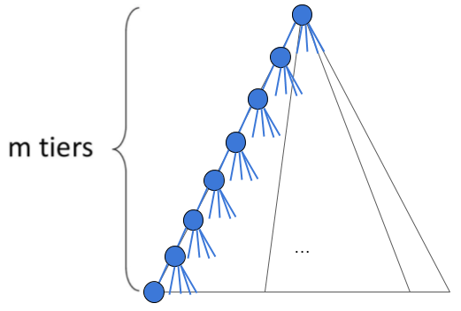
Time: In the worst case, DFS may search all other potential paths in the search tree before finding the solution. The size of this tree is \(O(b^m)\).

Space: Unlike BFS, DFS only keeps the "current" path it's considering on the frontier at a given time. Each level it traverses down the search tree, DFS expands (and adds to the frontier) up to \(b\) nodes, making the space complexity \(O(bm)\).
Completeness: Without keeping track of explored nodes, DFS can get stuck in an infinite loop visiting the same nodes again and again. Thus it only terminates when using graph search.
Optimality: DFS is not optimal. Try to think of a simple example where this is the case.
Similarly to BFS, you could also think of DFS as using a priority queue where the priority is the number of edges in the path, but instead you would pull off the path with the highest number of edges first. Once again, this allows for tie breaking between paths with the same number of edges, but it also has the flaw in that it allows for replacements of paths in the priority queue. Just like BFS, this is NOT an accurate representation of DFS because of this, and it is not representative of the DFS algorithm we use in class, so please use the algorithm presented in class, not a priority queue when running DFS.
UCS
Time: Since UCS follows path costs rather than depth levels, we bound the depth of the optimal solution by \(s \le \lfloor C^* / \epsilon \rfloor\) (as this is the total cost / minimum cost of one edge). Thus it must visit \(O(b^{\lfloor C^* / \epsilon \rfloor})\) nodes.
Space: Similar to BFS, UCS' space complexity is equal to its time complexity because it must keep track of all paths along the current cost contour as it visits nodes.

Completeness: UCS will get stuck in an infinite loop if there is a loop of zero-cost edges, so all edge costs must be \(> 0\).
Optimality: Note that UCS assumes no edges have negative cost - otherwise, it's possible that UCS would exclude an optimal path which has a high positive cost in its earlier edges (but a negative cost later on).
So assuming all edges are non-negative, because nodes are expanded in increasing cost order, when the algorithm gets to a goal node, it must be the lowest cost goal (i.e., must have reached it via the optimal path).
Iterative Deepening
Time: IDS has the same time complexity as BFS, since we are now bounded by the solution's depth level \(s\) (we'll never go deeper than \(s\)).
Space: IDS has the same space complexity as DFS, as we're literally running DFS as a subprocess.
Completeness: Since we’re bounded by depth, IDS doesn't fall into the same stuck-in-a-loop trap that DFS does, and will always terminate.
Optimality: UCS also finds the shallowest goal, which is the optimal goal if all edge costs are equal.
Note: While a ton of repeat work is done/space is used in IDS for the lower “failed" depth levels, we can simply consider the work done (space used) at the solution’s depth level (thanks big-O!), because this is where the bulk of the work (space) is, and # of nodes increases exponentially as we go down the search tree.
The time and space complexities of heuristic-based searches depend heavily on the heuristic chosen (surprise, surprise). The listed bounds are worst case scenarios.
Greedy
Time: In the worst case, greedy may visit all nodes in the graph before finding a goal. Thus the time complexity is \(O(b^m)\).
Space: In the worst case, greedy search could keep all paths of the nodes visited on the frontier - thus the space complexity is also \(O(b^m)\).
Completeness: With certain heuristic values, greedy search could get stuck in a loop of expanding the same nodes - try making an example!
Optimality: Without the right heuristic values, greedy search is not guaranteed to find the optimal solution.
A*
Time: Recalling the idea of cost contours from UCS, A* instead visits nodes along \(f\)-contours. In the worst* case, suppose we have a constant heuristic (\(h\) estimates that all nodes are equally far away from the goal). Then A* functions like UCS, expanding all nodes shallower or at the same depth level of the solution: \(O(b^{\lfloor C^* / \epsilon \rfloor})\).
*One could construct a misleading/adversarial heuristic which actually forces A* to expand all nodes before finding the goal. We’re not really interested in such cases in this class, so we’ll ignore such analyses here.
Space: In the case of constant heuristic, A* must keep all nodes and paths up until the solution’s contour in the frontier at once. Thus the space complexity is also \(O(b^{\lfloor C^* / \epsilon \rfloor})\).
Completeness: A*, no matter the heuristic or tree/graph search, will always find a solution as long as no edge costs are negative (otherwise it would get stuck in a loop of ever-decreasing \(f\) values) and terminate.
Optimality: A* with tree search + an admissible heuristic leads to an optimal solution by mechanics of A* - no other node has a \(f(n) = g(n) + h(n)\) value lower than the one being currently expanded. Since h is admissible, the first path to the goal found must be the cheapest of all possible paths.
With graph search, however, since we have the potential for cycles (and the explored set to account for that), we need the additional constraint that no "heuristic-estimated step cost" (difference in heuristic value between two nodes) overestimates the actual cost of that edge. If this is not satisfied, we could potentially expand some path A \(\rightarrow\) C when A \(\rightarrow\) B \(\rightarrow\) C would’ve been cheaper, and we wouldn’t be able to revisit C and find this cheaper path after exploring C - thereby returning a suboptimal solution.
(Consider the following example with heuristic values \(h(A) = 7, h(B) = 6, h(C) = 2, h(G) = 0\). Let A be our start state, and G the goal. Note that consistency is broken between B and C, because cost(B to C) \(< h(B) - h(C)\).).
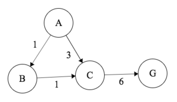
If the heuristic were consistent, however, such a case would not happen, and the algorithm is guaranteed to be optimal.
Adversarial Search
Games
There are many different kinds of games. In this course, we will be covering "standard" games, which are deterministic, observable, two-player, turn-taking, and zero-sum.
Two types of games are:
General games: agents have independent utilities.
Zero-sum games: agents have opposite utilities. A gain in utility for one player will result in a decrease in utility for others.
Our goal is to define a strategy/policy that recommends a move for every possible eventuality.
Minimax, Expectimax, Expectiminimax
Minimax is typically used for two-player, zero-sum game in which one player is trying to maximize their utility and the other player is trying to minimize their utility.
The value and action for a maximizing node are:
- \(V(s) = \max_{a} V(s')\)
- â = argmax\(_a V(s')\)
The value and action for a minimizing node are:
- \(V(s) = \min_{a} V(s')\)
- â = argmin\(_a V(s')\)
Where \(s'\) = result(s, a), i.e., the resulting state when an agent takes action \(a\) from state \(s\).
In the case that the game is not two-player or zero-sum, minimax can be generalized. In this scenario, each node will have a tuple of utility values, representing the utility for each player. Each player will maximize their own component.
Minimax Runtime
We can think of minimax as an exhaustive DFS. Thus, the space and time complexities are as follows:
Time: \(O(b^m)\)
Space: \(O(bm)\)
Chance Node
Chance nodes are nodes that return the expected value over all possible resulting states. For example, an expectimax game consists of chance nodes and maximizing nodes. The maximizing nodes will choose an action with the highest expected value.
The expected value of a node is the average of the values of the different outcomes weighted by the probability of that outcome. The value of a chance is thus given by \(V(s) = \sum_{s'}P(s')V(s')\).
Bounded Lookahead
In reality, it is often infeasible or inefficient to search to all the leaves. Thus, one solution would be to search only to a preset depth limit or horizon. We would use an evaluation function to determine a return value for non-terminal positions instead.
Evaluation functions score non-terminal nodes in depth-limited search. Ideally, we want a function that will return the actual minimax value of the position.
In practice, these functions are often a weighted linear sum of features, ie. EVAL(s) = \(w_1f_1(s) + w_2f_2(s) + ... + w_nf_n(s)\).
Alpha-Beta Pruning
Alpha beta pruning is an algorithm that aims to decrease the number of nodes minimax needs to evaluate.
For each node, we keep track of two values:
\(\alpha\): the best option so far for any MAX node on this path
\(\beta\): the best option so far for any MIN node on this path
The algorithm at a maximizing node looks as follows:
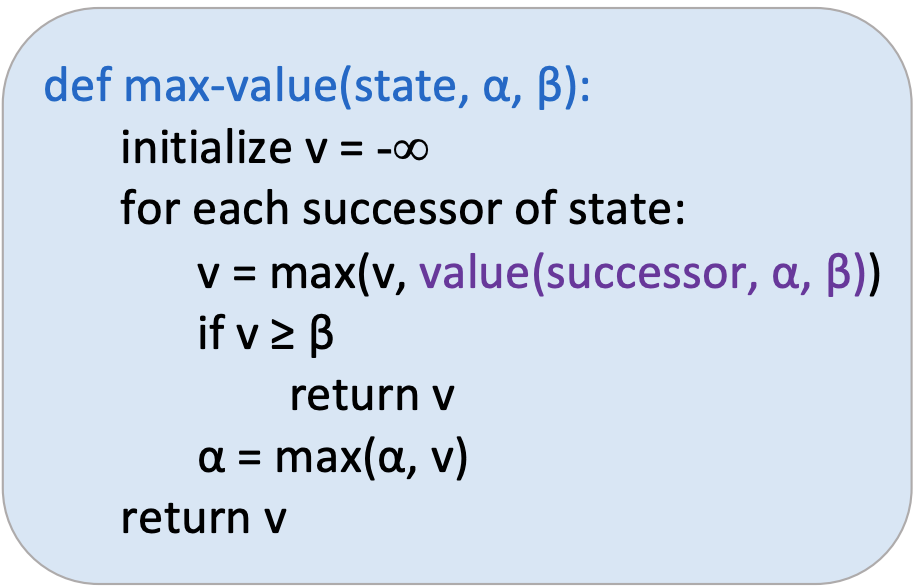
The algorithm at a minimizing node looks as follows:
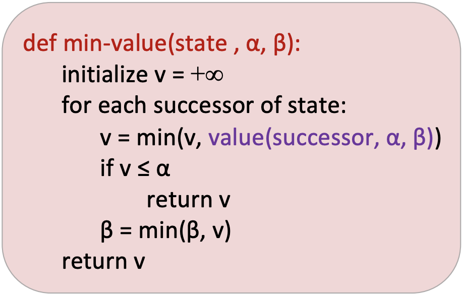
Important: Alpha beta pruning has no effect on the minimax value computed for the root. The ordering of child branches improves the efficiency of pruning. With "perfect" ordering, the time complexity becomes \(O(b^{m/2})\).
The following is a table to summarize \(\alpha\beta\) pruning.
\[\begin{array}{|c|c|c|c|}
\hline
& x\leq \alpha & \alpha < x < \beta & x \geq \beta \\
\hline
\mbox{Maxie} & \mbox{Ignore} & \mbox{Update } \alpha & \mbox{Prune} \\
\hline
\mbox{Minnie} & \mbox{Prune} & \mbox{Update } \beta & \mbox{Ignore}\\ \hline
\end{array}\]
Example
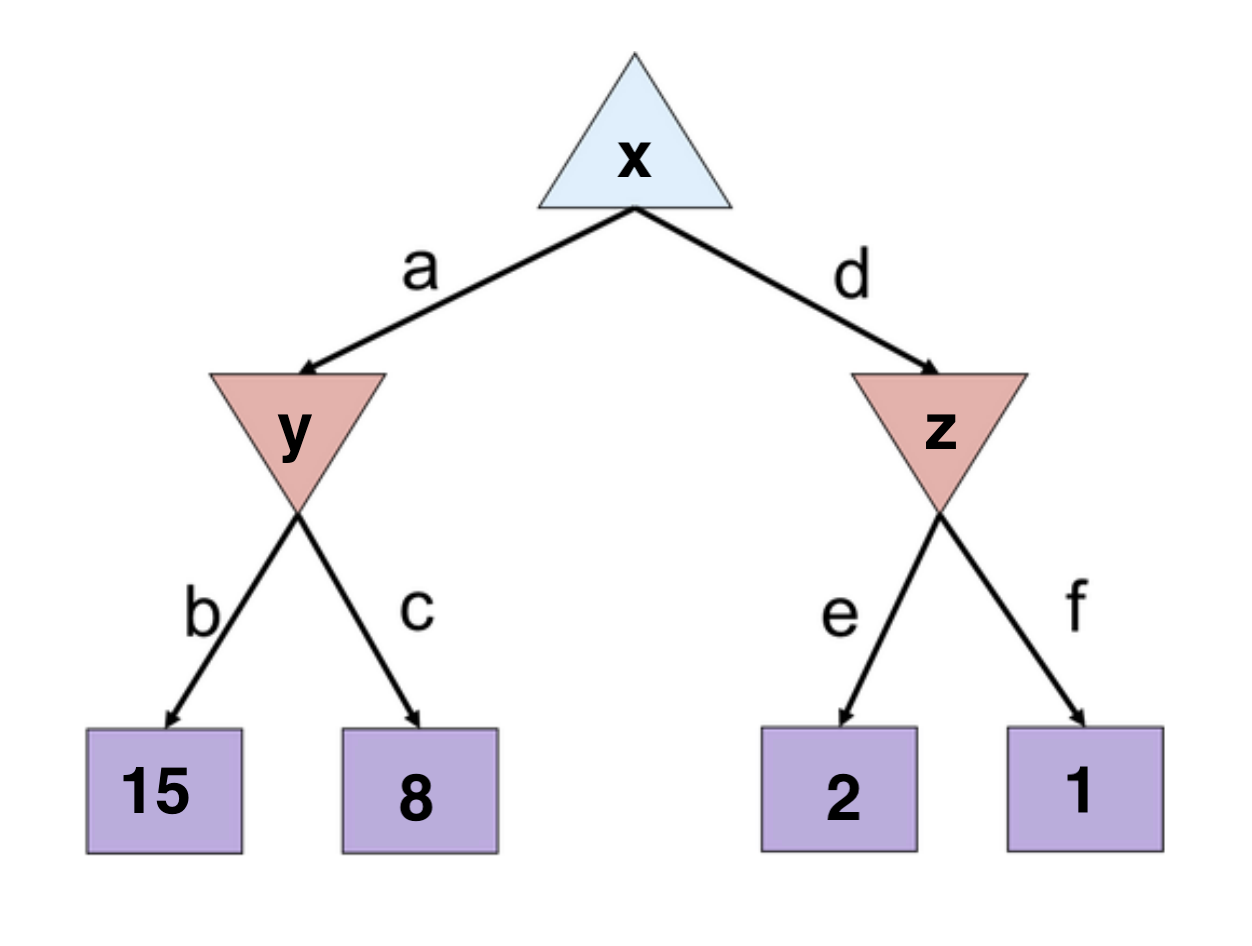
Initialize \(v=-\infty\), \((\alpha, \beta) = (-\infty, \infty\)) for node x because it is maximizing
Initialize \(v=\infty\), \((\alpha, \beta) = (-\infty, \infty\)) for node y because it is minimizing
Traverse down branch b and return 15 to y. Update v=15, \(\beta=15\) for y. The updated \(\alpha\beta\) values for y are \((-\infty, 15\))
Traverse down branch c and return 8 to y. Update v=8, \(\beta = \min(15, 8) = 8\) for y. The updated \(\alpha\beta\) values for y are \((-\infty, 8\))
Node y returns v=8 to node x. Update v=8, \(\alpha=8\) for x. The updated \(\alpha\beta\) values for x are \((8, \infty\))
Traverse down branch d and initialize \(v=\infty\), \((\alpha, \beta) = (8, \infty\)) for node z. (Note: the \(\alpha\beta\) values are passed down from x)
Traverse down branch e and return 2 to z. We see that this value is outside of the \(\alpha\beta\) range (ie. \(2 \leq \alpha\)). Thus, we prune the rest of node z's child branches.
Node z returns 2 to x. x's value remains 8 and x returns 8.
Let us think about what just occurred intuitively. When node x visited its left branches, a value of 8 was returned. Then it traverses down d-e and sees the value 2. x knows that it can guarantee at least a value of 8 by going down the left branch. However, x also reasons that it can only get a value of at most two by going down the right branch.
If the unvisited branch (f) has a value \(> 2\), then z will return 2 since z is trying to minimize
If the unvisited branch has a value \(\leq 2\), then z will return that value.
Therefore, x knows that it will get a better deal by traversing down branch a and does not care about the value down branch d-f. This allows us to prune branch f.