Differentiable Refractive Ray Tracing
Exploring the GRIN Lens Design Space
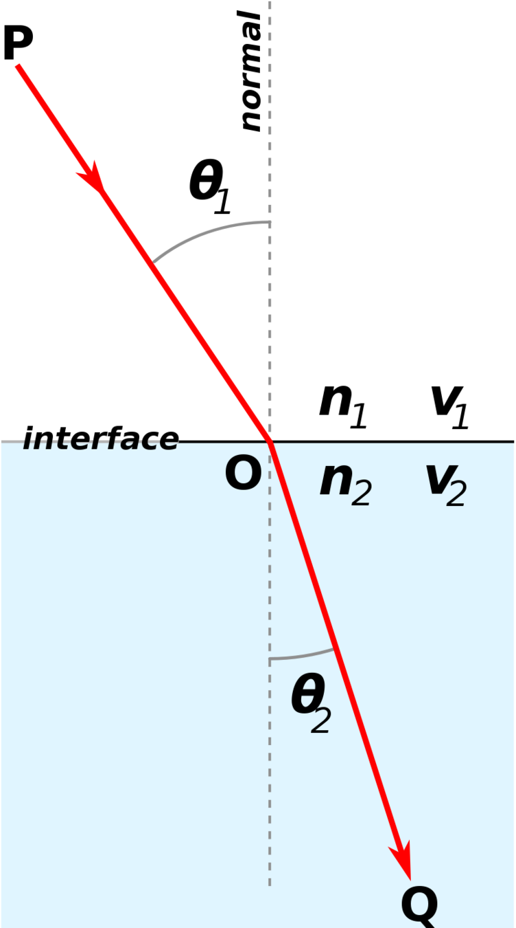
Refraction

Ray Tracing, Snell's Law
Gradient Index Ray Tracing
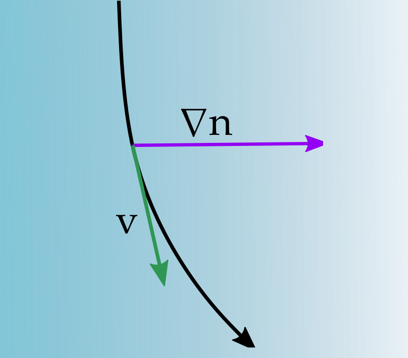

What about gradient interfaces?
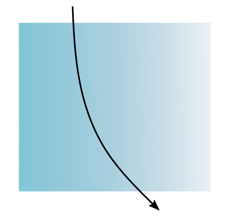

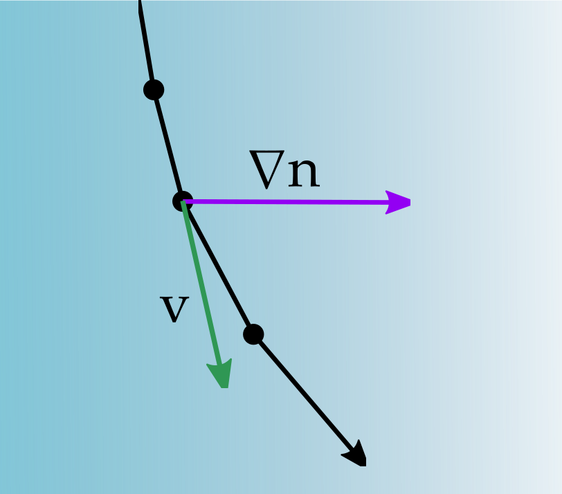
Gradient Refractive Fields
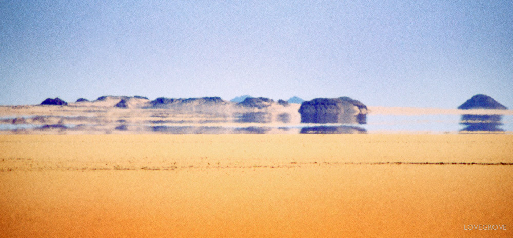
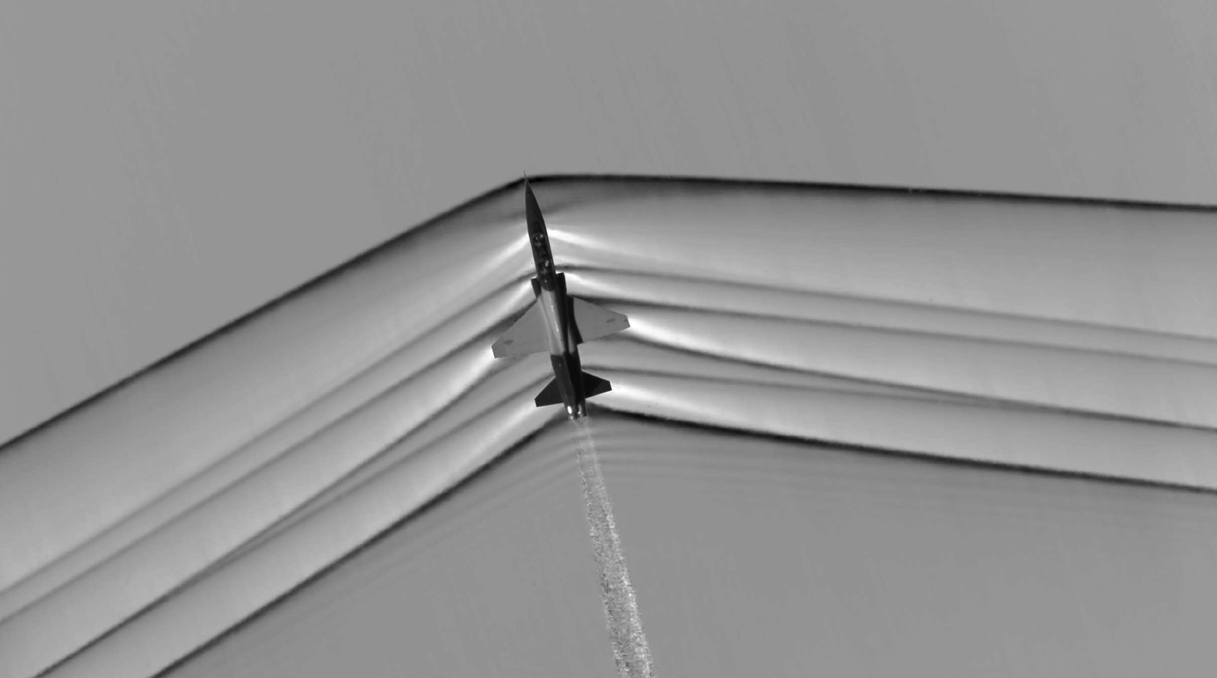
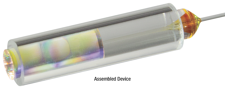
https://www.thorlabs.com
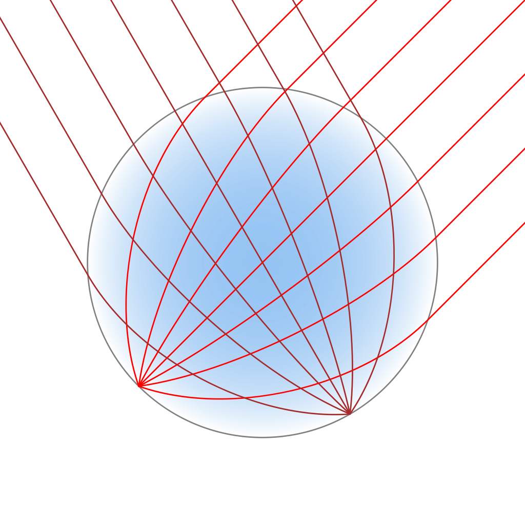
Luneburg Lens
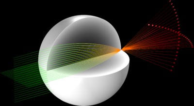
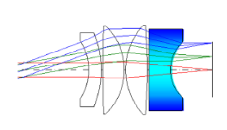
Why GRIN Lens?
GRIN Lenses have many more degrees of freedom over traditional lenses.
What sort of effects can we achieve in this space? What are the limitations?
Mostly a theory question
What can GRIN Lenses do that traditional refractive lenses cannot? Vice Versa?
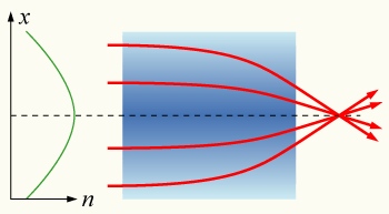
Pretty ill-defined question, so instead...
If we have an objective, what profile achieves it?

We know some (Luneburg, Maxwell, etc.), but what about other objectives?
Outline
- Forward Tracing
- Inverse Problem
- Solve via Autodiff
- Adjoint Method
- Experiments
Ray Tracing Equations

Simulating GRIN Fields
The Problem Statement

Assuming our desired inputs, what refractive field generates the desired output?
The Problem Statement
(We will ignore wavelength)
The inverse formulation
The cost objective can be anything as long as its a function of \(x\) and \(v\)
Solve it with autodiff!
Initial Conditions
\(x_o, v_o\)
Refractive Field
\(\eta\)
Eikonal Tracer
Cost Objective
Backprop
Gradient
An example problem
An example is an image formation model, where each ray carries constant irradiance
The goal is to have multiple images based on direction
2 Images, 2 Directions
Collimated Sources
Sensors
\(\eta\)
Autodiff Results
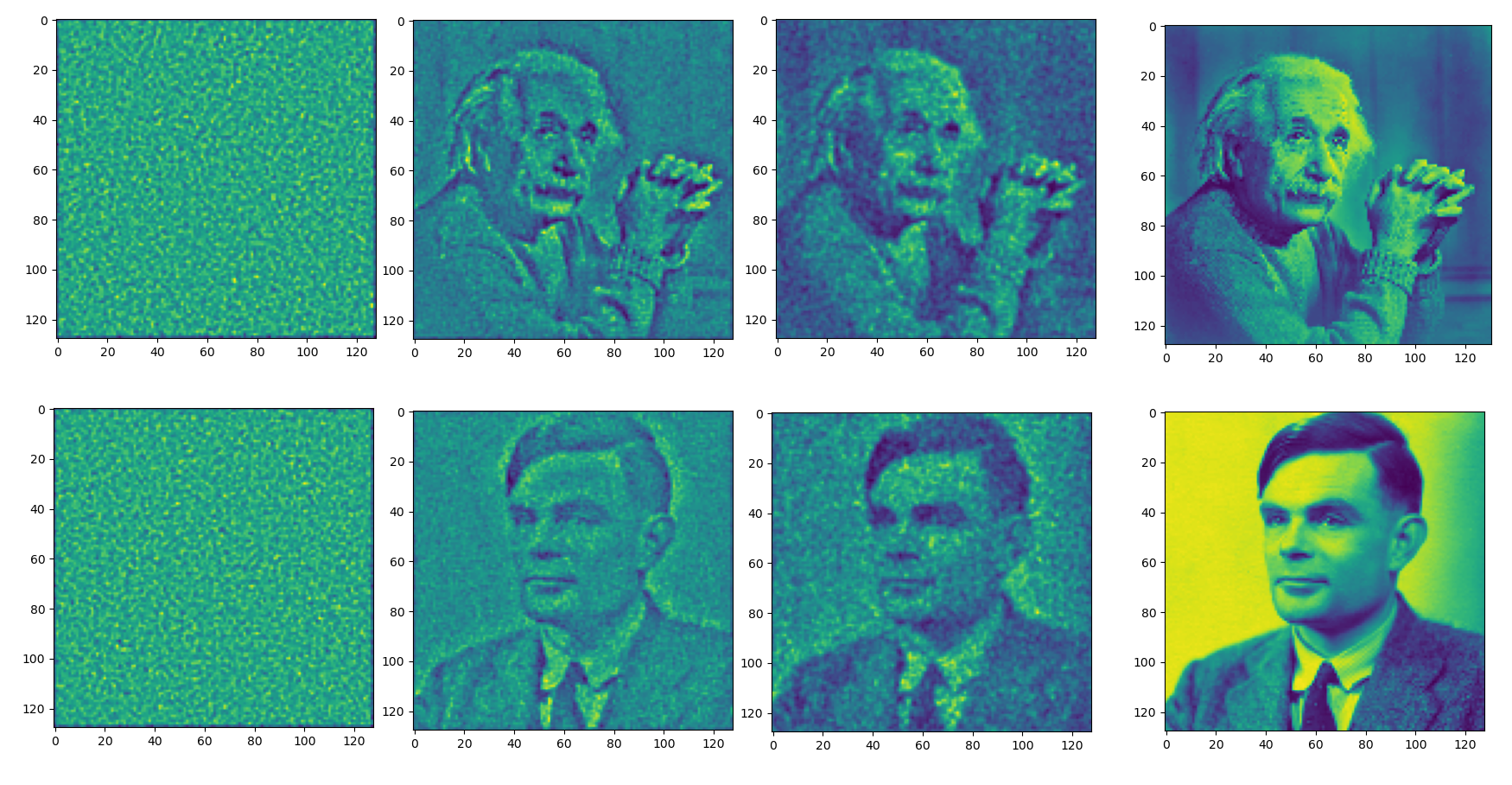
Ground
Truth
Iter 0
Iter 20
Iter 300
Autodiff is expensive...
- 128x128 pixel target images
- 10 samples per pixel
- 128^3 resolution cube
- ~5s per iteration
-
~12GB GPU memory usage
- forward trace + backprop
PyTorch Implementation:
AD Graph
Every integration step is a "layer" in the graph
\(\Delta s\)
\(\Delta s\)
\(\Delta s\)
Autodiff is step size dependent
Each time step in the simulation adds to the computation graph.
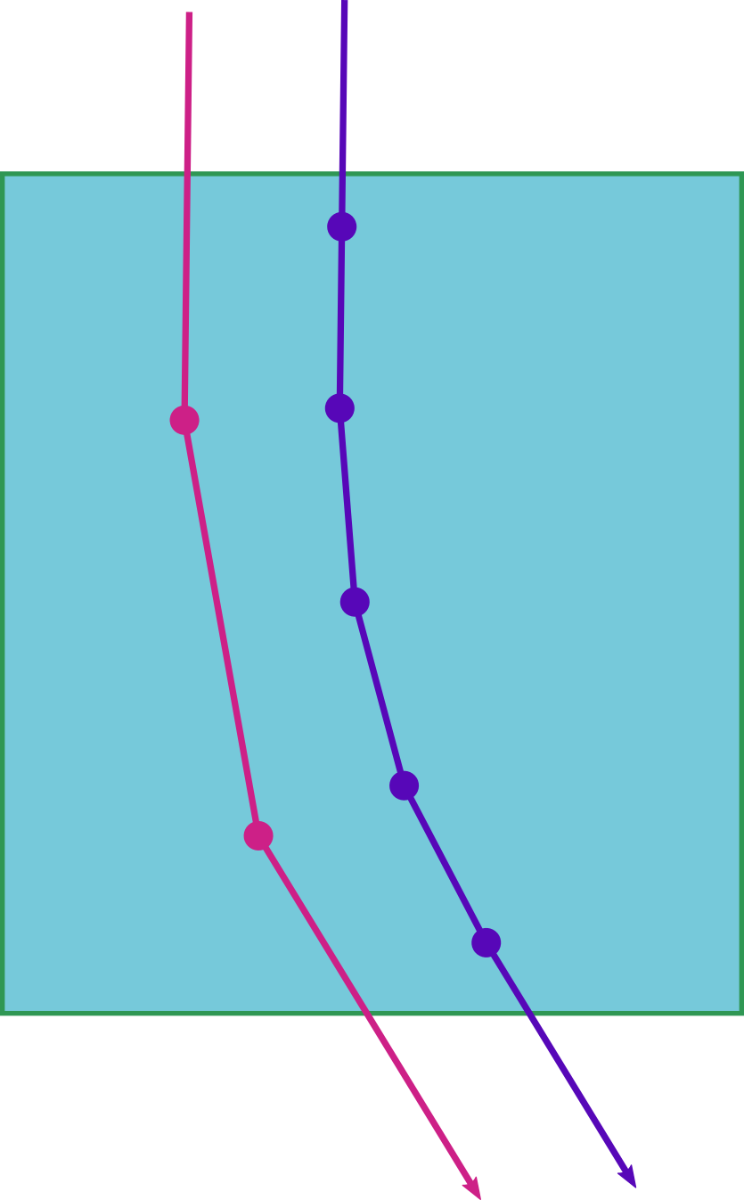
Halving the step size effectively doubles the computation graph!
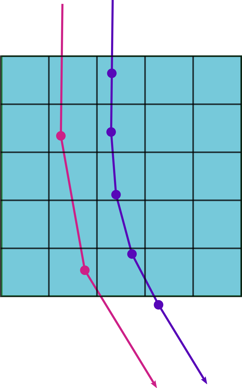
Higher resolution requires smaller step size
Too low of a step size means the volume itself will be undersampled.
Adjoint State Method
A method for computing the derivative of interest via a set of partial differential equations
Gradient from Adjoint State
Calculating the adjoint state \(\mu\) gives us the value needed for the derivative of interest
With this value, we can use a gradient based optimizer like Adam, SGD, BFGS, etc.
Adjoint via Backtracing
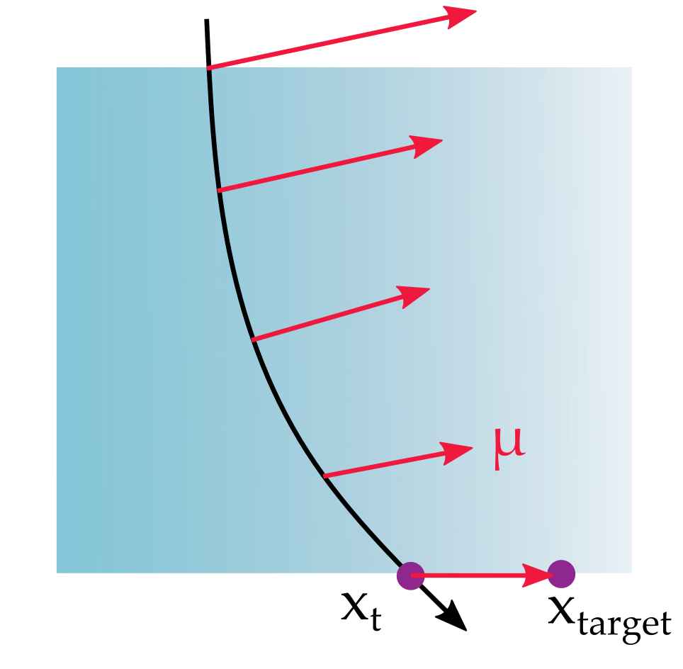
\(\mu\) can be thought of as the error vector at the boundary being parallel transported back through the volume
Adjoint via Backtracing

We still need the path for the adjoint state, since its defined on the path.
Naively, this means that we have to save the whole path, which has the same problem as before.
Time-reversibility

The optical paths of the rays are "symplectic" or reversible.
Same experiment
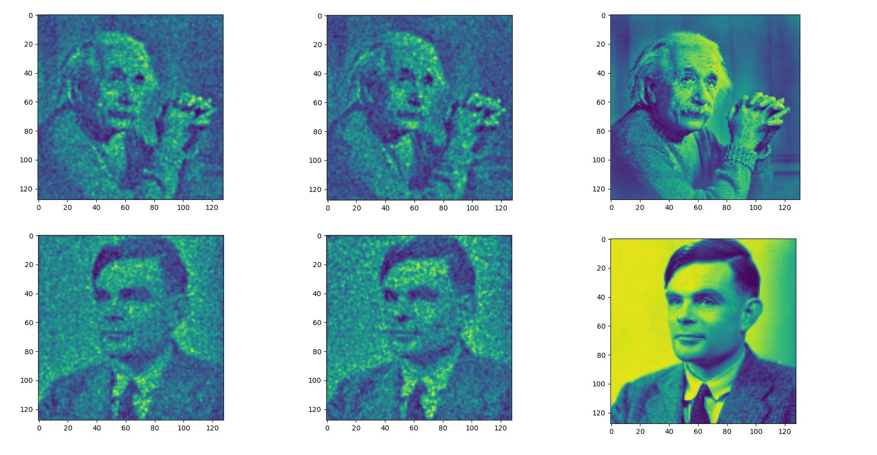
Ground
Truth
Autodiff
Adjoint
Performance Numbers
AD Implementation:
- ~5s per iteration
- ~18GB GPU mem
- 128x128 pixel target images
- 10 samples per pixel
- 128^3 resolution cube
Adjoint Implementation:
- ~1s per iteration
- ~2GB GPU mem
Larger and more accurate simulations
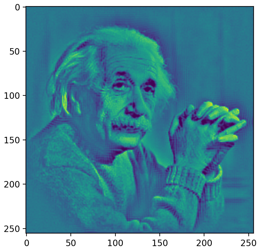
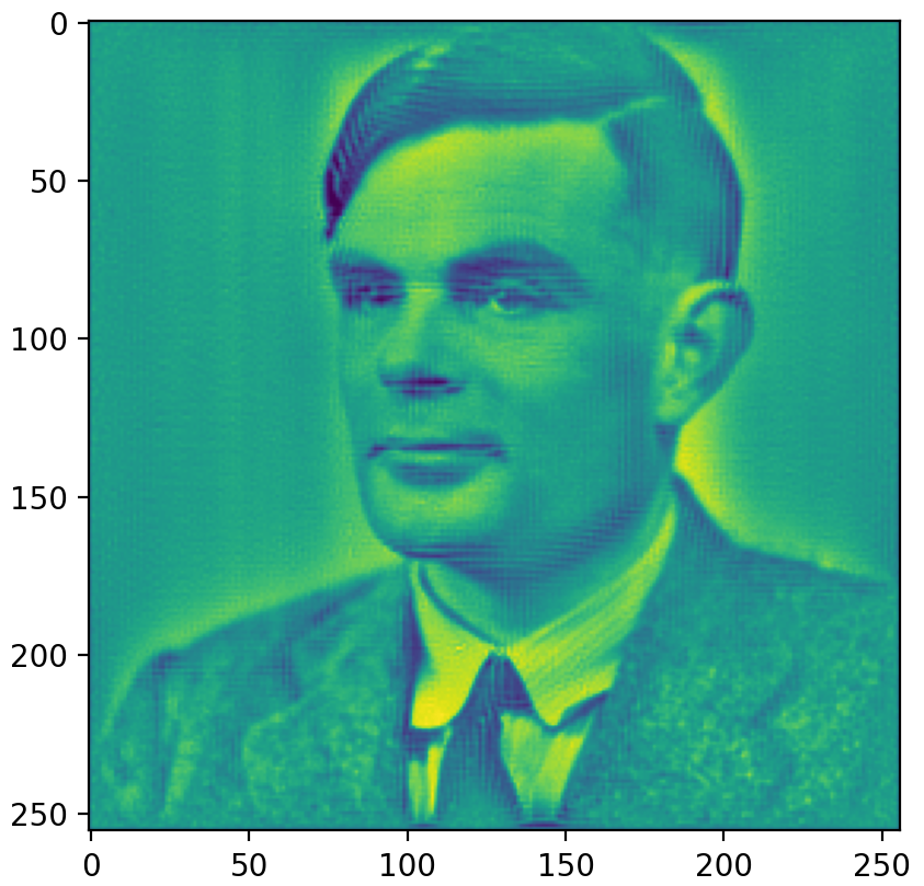
AD can also achieve these results, it would just take much longer and use more memory.
Adjoint Replaces AD
Adjoint
Tracer
Different Design Tasks
Near and Far Fields
Collimated Source
Near-Field Sensor
\(\eta\)
Far-Field Sensor
Near and Far Fields
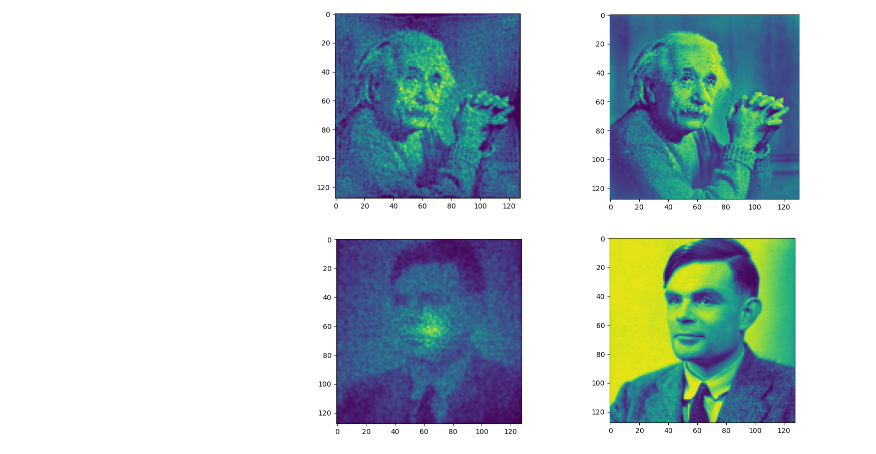
Optimization
Ground Truth
Near
Far
Caustic Designs
Same near-far setup, but use a geometric cost objective instead
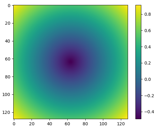
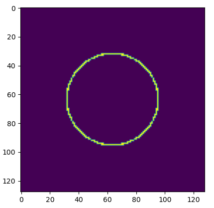
desired image
signed distance field
Caustic Designs

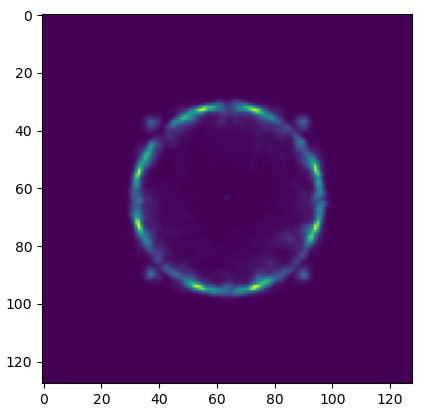
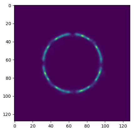
Near Field
Far Field
Ground Truth

Volume
Caustic Designs (problem)


Near Field
Far Field
The energy distribution isn't uniform. That isn't a constraint in the optimization.
As long as the ray reaches the circle, the loss will go to zero.
Luneburg Reconstruction
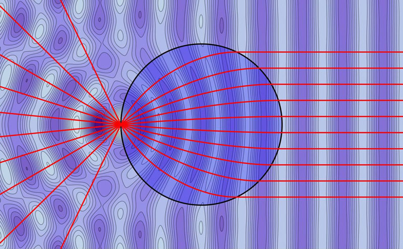
The Luneburg lens can be defined by a geometric property rather than an index profile.
Luneburg Reconstruction

Luneburg Reconstruction
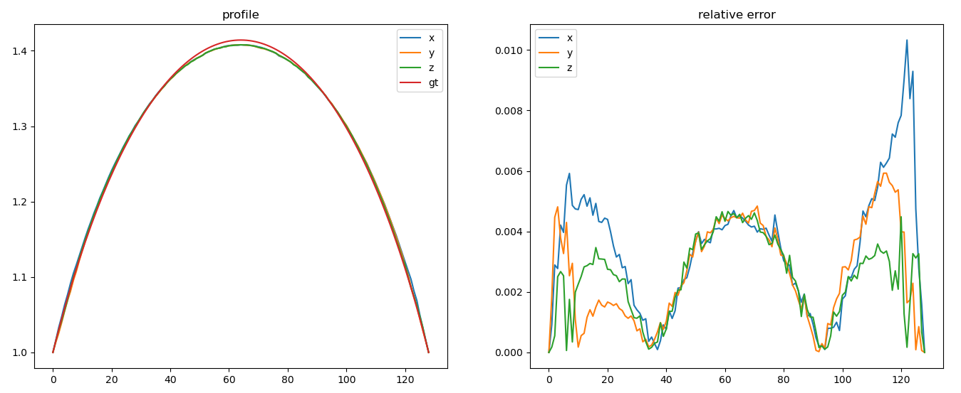

It works! We can match the actual Luneburg profile with just the geometric description.
Closing Thoughts
- Can't handle discrete interfaces.
- Don't account for real world fabrication constraints
- Extensions include:
- polarization
- wavelength dependence
More Examples?
What sort of things would be cool to see?
What other experiments should I try?