Hypothesis Testing
Key ideas:
- How to prove or disprove a hypothesis/claim by sampling data.
- How to compare two classifiers.
- How to sample data for this purpose.
Outline
The basic idea behind hypothesis testing is as follows: a claim has been made about some statistic. Typical examples:
- For instance, a politician may claim that more than 50% of the population will vote for him.
- A company that makes bulbs claims that the average life expectancy of their bulbs is 1000 hours.
- The census department claims that the percentage of voters among men is no different than the percentage of voters among women.
- Your employer claims that the new classifier you have developed is no better than the one the company is already using.
Lets call this claim the Null Hypothesis, usually represented by $H_0$.
You would like to challenge this claim (the null hypothesis $H_0$).
Your counter belief for four above cases may be that
- The actual support for the politician is less than 50%,
- The actual life expectancy of the bulb is less than 1000 hours,
- The fraction of voters is NOT the same among men and women,
- Your classifier is better.
We will call your counter belief the Alternate Hypothesis, and represent itas $H_a$.
Note that the alternate hypothesis doesn't really make a claim of its own. Its primary objective is to reject a default claim made by someone else -- the purpose is to reject the null hypothesis.
To evaluate the validty of the null hypothesis we sample data, and run a test on this sample to verify if we can reject the null hypothesis.
The test itself consists of computing a statistic $Y$ from the sample and checking if its value falls within a rejection region $R$ (which is typically defined as one of $Y \leq \theta$, $Y \geq \theta$, or $|Y| \geq \theta$ for some threshold $\theta$). If the value of the computed statistic $Y$ falls within this rejection region, we decide that the null hypothesis $H_0$ can be rejected, if not, we cannot reject $H_0$.
In rejecting or accepting the null hypothesis $H_0$, we do not want to make errors (i.e. rejecting $H_0$ when it is actually correct, or accepting $H_0$ when it is actually wrong). If rejection region $R$ (or threshold $\theta$) is improperly chosen, these errors can become unacceptably likely. So, when specifying the rejection region $R$ we chose it carefully, so that the probability of error is small. In practice, we first specify the largest probability of error that is acceptable (typically a value such as 0.05), and then chose $R$ such that the error probability meets our specification.
Let us now look at this in more detail.
Basic Formalism
Formally, a hypothesis testing procedure must specify the following four terms
- A null hypothesis $H_0$,
- An alternate hypothesis $H_a$,
- A statistic $Y$ that we will compute from a set of data samples,
- A rejection region $R$ for $Y$, typically specified by a threshold $\theta$.
If the statistic $Y$ falls within the rejection region $R$, we will reject the null hypothesis and accept our alternate hypothesis. Otherwise we not have established sufficient reason to reject the null hypothesis.
Note that this does not necessarily mean that the null hypothesis is correct; it only means that we do not have the evidence needed to reject it.
Errors
We are liable to make two kinds of errors when we run a hypothesis test:
- Type 1 Error: We reject the null hypothesis when it is in fact true.
- Type 2 Error: We accept the null hypothesis when it is in fact false.
Type 1 Errors
Type 1 errors happen if the statistic $Y$ falls within rejection region $R$ even though $H_0$ is true. There is always a likelihood of this happening.
To illustrate, consider an example where we test the fairness of a coin. The null hypothesis $H_0$ is that the coin is fair. Our alternate hypothesis is that in fact it is not fair and $P(heads) > P(tails)$.
To evaluate the hypotheses we conduct a test in which we flip the coin 10 times and count the number of heads. We figure that if 8 or more of these tosses turn up heads, we can reject the hypothesis that the coin is fair. So here our test samples are the 10 tosses, the statistic $Y$ is the number of heads, and the rejection region is $Y \geq 8$. Clearly, this is a reasonable test. But how often will this test erroneously tell us that a coin is not fair when it is actually fair?
To evaluate this, consider repeating the test (of flipping the coin 10 times) a very large number of times on a fair coin. How frequently will the fair coin give us 8 or more heads in 10 tosses? Its easy for us to compute this number: the probability that a fair coin (with P(heads) = 0.5) will give us 8 or more heads in 10 tosses is given by $P( Y \geq 8| P(heads) = 0.5) = \sum_{Y=8}^{10} {10 \choose Y} 0.5^Y 0.5^{10-Y} = 0.0546875$.
The probability of a type 1 error in this test is 5.46875%. This is the fraction of times we would conclude that the fair coin is unfair with $P(heads) > P(tails)$ if were to use our test.
In general, the probability of a type I error may be interpreted as the fraction of times we would end up rejecting the null hypothesis, even though it is actually true, if we were to repeat our test using our rejection criterion a very large number of times.
We always want the probability of a type 1 error to be low. We will generally refer to the probability of a type 1 error as $\alpha$.
\[
P(Type\; 1\; Error | H_0) = \alpha
\]
The figure below illustrates this with a figure.
The converse of the probability of type 1 error is also called the confidence in the test. Thus, if $\alpha = 0.05$, we can also claim that we have 0.95 (or 95%) confidence in the test, which is to say that we are 95% sure that the test wont reject the null hypothesis by mistake.
Type 2 Error
Type 2 errors happen if the statistic $Y$ falls outside the rejection region $R$ and we accept $H_0$, even though $H_0$ is false. Again, this is a distinct possibility.
To understand, lets revisit the above example. We suspect that the coin is not fair, and that $P(heads) > P(true)$. So we conduct a test where we flip the coin 10 times and decide that the null hypothesis $H_0$ (that the coin is fair) must be rejected if we obtain 8 or more heads.
Consider now that the coin is in fact biased and has P(heads) = 0.7. How frequently will this coin pass the test for a fair coin? The coin is accepted as a fair coin if we get fewer than 8 heads, according to our test. The probability of this happening can be computed as $P(K < 7 | P(heads) = 0.7) = \sum_{K=0}^7 {10 \choose K} 0.3^K (1 - 0.3)^{10-K} = 0.6172$.
The probability of a type 2 error for a coin with $P(heads) = 0.7$ is 0.6172. This is the fraction of times we would conclude that this biased coin is fair if were to use our test.
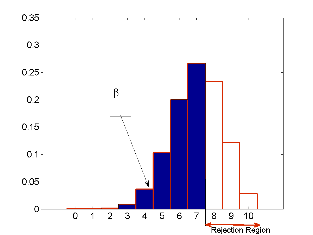
The figure below illustrates this with a figure.
In general, the probability of a type 2 error may be interpreted as the fraction of times we would end up accepting the null hypothesis, even though the alternate hypotheis is true, if we were to repeat our test using our rejection criterion a very large number of times.
We will generally refer to the probability of a type 1 error as $\beta$.
\[
P(Type\; 2\; Error | H_a) = \beta
\]
Note that in order to compute $\beta$, we need to know the true value of the parameter that the null hypothesis defines. In our examples, this would be $P(heads)$. At the least, the alternate hypothesis must hypothesize a value of this parameter, instead of merely rejecting the null hypothesis (so that we can use it to compute $\beta$). In general, this wont be possible however, and $\beta$ cannot be known. We can however make some statements about trends in $\beta$ as we will see below.
Error tradeoffs
Our primary control over the probabilities of type 1 and type 2 errors is through the rejection region $R$ and the number of samples $N$ in the test. Lets consider these in turn.
Controlling error through the rejection region
The rejection region $R$ is the range of values that the statistic must take in order to reject the null hypothesis $H_0$. If the statistic falls outside the rejection region, the null hypothesis must be accepted. Lets refer to this region as the acceptance region (this is not standard terminology) and represent it by $\bar{R}$.
$\alpha$, the probability of type 1 error, and $\beta$, the probability of type 2 error, can both be modified by changing the rejection region. However, here we face a tradeoff.
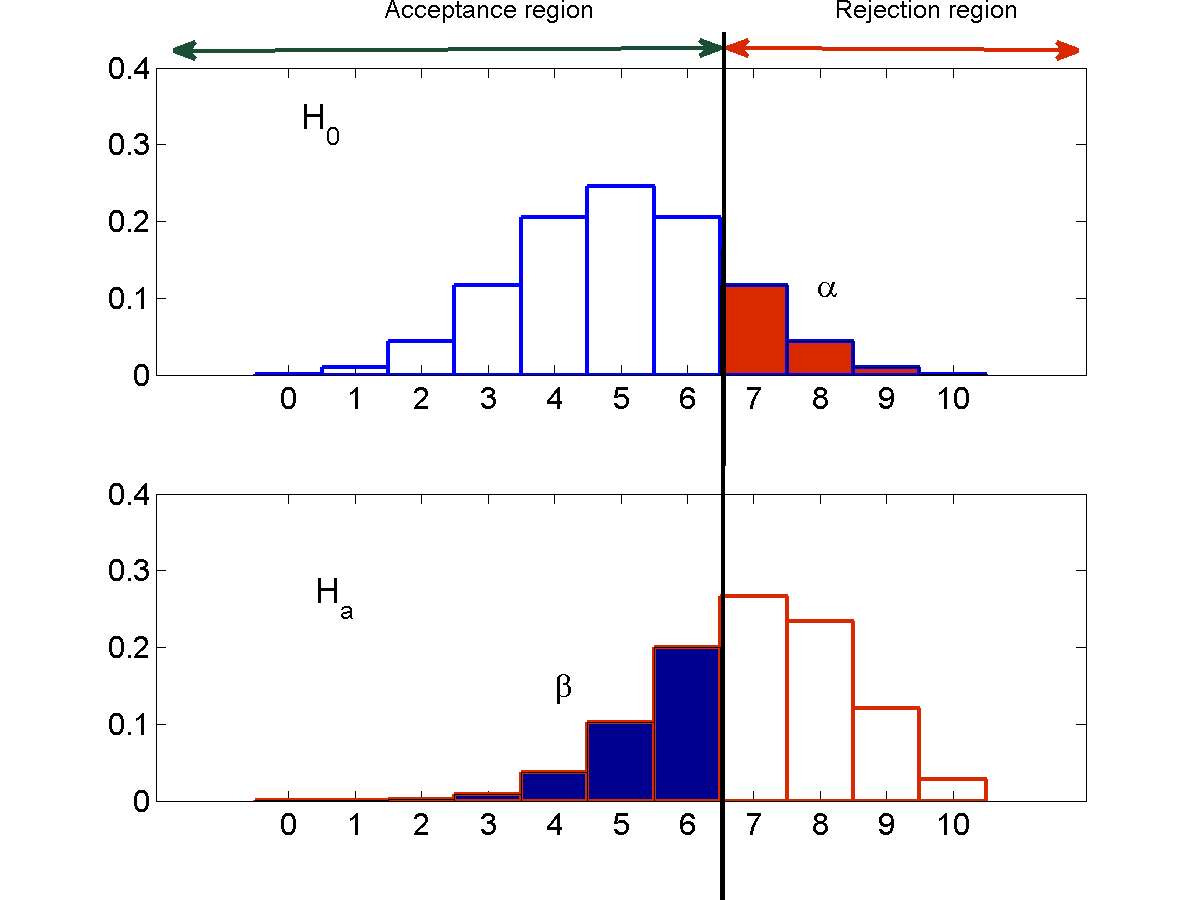
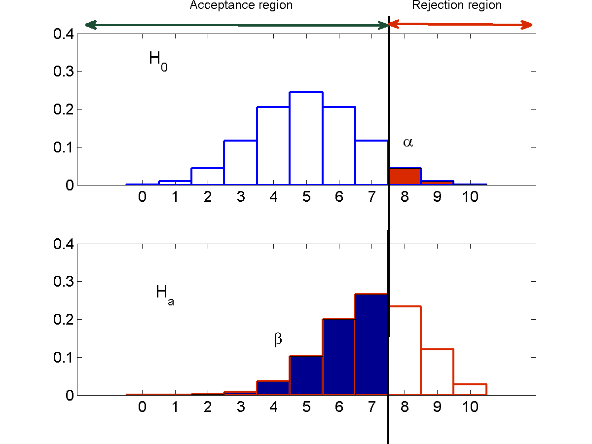
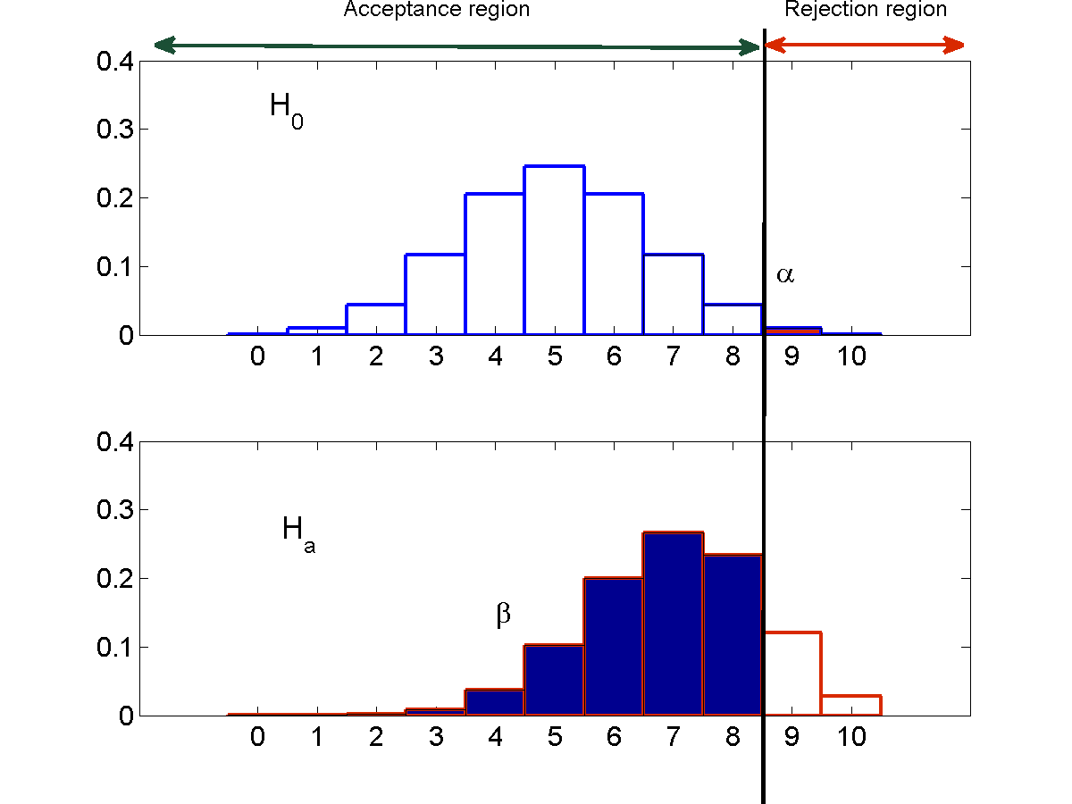
Type 1 errors occur only when the test statistic falls within the rejection region $R$. If we reduce $R$, the probability of type 1 errors will naturally decrease. On the other hand, type 2 errors only occur when the test statistic falls outside the rejection region, i.e. when it falls in the acceptance region $\bar{R}$. In order to reduce type 2 error, we must reduce $\bar{R}$.
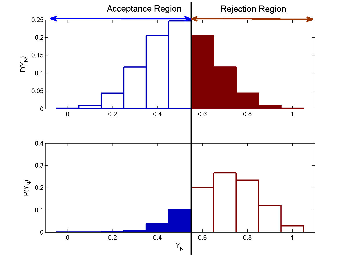
Thus, modifying the rejection region to decrease the probability of type 1 error, $\alpha$, will result in an increase in $\beta$ and vice versa. This is illustrated by the figure below, using the coin example from earlier.
Thus, if the number of samples $N$ is fixed, we cannot decrease both $\alpha$ and $\beta$. In any case, unless the true value of the parameter that the null hypothesis is about ($P(heads)$ in our example) is known, $\beta$ cannot be computed anyway. Thus, in situation where $N$ cannot be controlled, or when the alternate hypothesis does not specify a particular value for $P$, we generally focus on $\alpha$, the probability of type 1 error, and ignore type 2 errors.
Controlling error through the number of samples $N$
There is a way of improving both $\alpha$ and $\beta$, at that is by increasing $N$, the number of samples in the experiment. To illustrate how, lets continue with our previous coin example.
We still want to test the null hypothesis $H_0$ that the coin is fair. Only, instead of a fixed sample size of 10 samples, let us now consider other sample sizes. We will have to modify our tests accordingly, however. For example, if our test when $N=10$ (ten tosses) is that the number of heads $K \geq 6$, for $N=100$ we would have to modify it to $K \geq 60$, or more generally, for $N$ tosses, we can use a rejection region of $K \geq 0.6N$.
To simplify matters, rather than modify the test for each $N$, we can instead normalize our statistic. I.e. instead of comparing the number of heads $K$ to a threshold, e.g. 6, we will compute a the normalized statistic $\bar{Y}_N = \frac{K}{N}$. We can now use a fixed test $\bar{Y}_N \geq 0.6$ in every case.
Note that the tests $K \geq 0.6N$ and $\bar{Y}_N \geq 6$ are strictly equivalent, and $P(K \geq 0.6N) = P(\bar{Y}_N \geq 0.6)$. The distribution of $\bar{Y}_N$ is identical to that of the distribution of the probability of $K$ heads in $N$ tosses, other than that the values over which the probability is defined will now go from $0, \frac{1}{N}, \frac{2}{N}, \cdots, 1$, rather than $0, 1, 2, \cdots N$. We can hence compute $\alpha$ and $\beta$ just as well from the probability distribution of $\bar{Y}$ under $H_0$ and $H_a$.
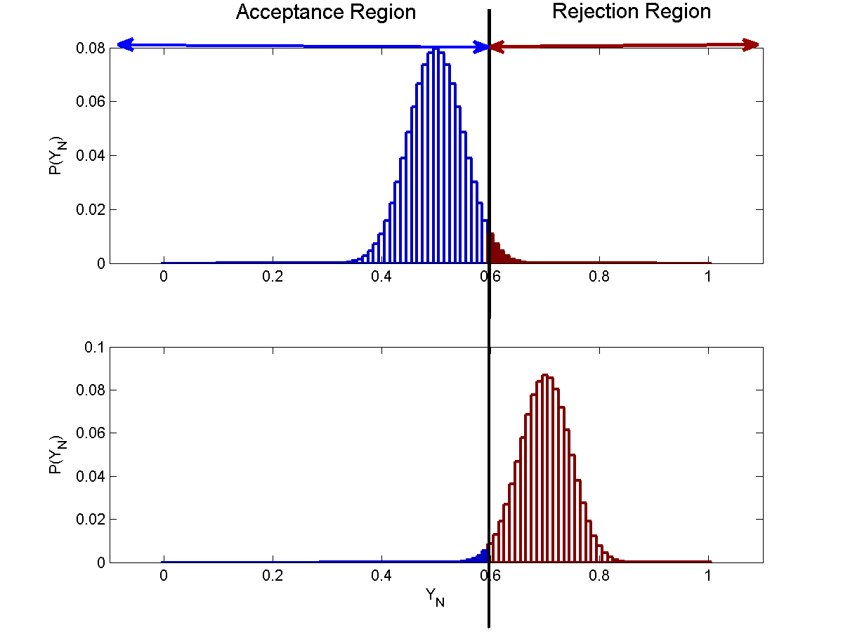
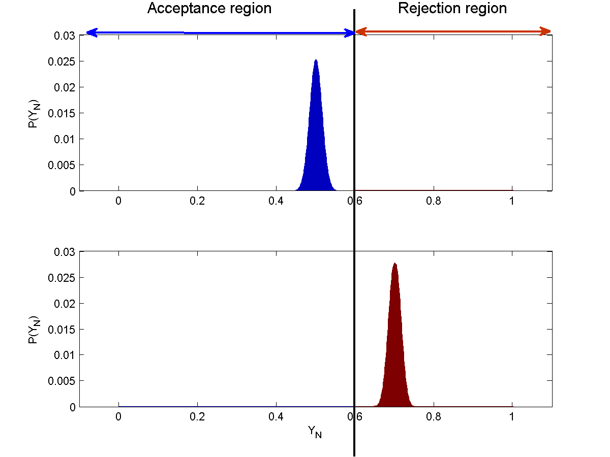
The figure below shows the distribution of $\bar{Y}_N$ for $N=10$, $N=100$ and $N=1000$.
From the above figures, we see that as $N$ increases the probabilities of both type 1 and type 2 errors falls.
To understand this, we note that $\bar{Y}$ is, in fact, a point estimate of $P(heads)$ under each of the two hypotheses, and, as we saw under the properties of point estimators, its variance shrinks with $N$. For a Bernoulli random variable whose variance is $P(heads)(1-P(heads))$, the variance of $\bar{Y}$ is $\frac{P(heads)(1-P(heads))}{N}$. As $N$ increases, the variance of this estimate shrinks.
As a consequence, the area of the probability distribution on the “wrong” side of the rejection threshold decreases with $N$, and both $\alpha$ and $\beta$ shrink.
In practice one does not usually have the information necessary to quantify $\beta$, so we attempt to obtain as many samples as we can, and choose the rejection region $R$ such that the probability of type 1 error falls below a threshold we deem acceptable. This is the format of most hypothesis tests. In some cases, however, we may have some information about $H_a$, in which case we can try to minimize $\beta$ as well.