Resource analysis of programs aims to infer their worst-case cost bounds. It has a number of practical use cases. For example, when executing a client’s program in cloud computing, a cloud-service provider (e.g., Amazon Web Services or Microsoft Azure) would like to to avoid both over-provisioning resources (which would reduce profits) and under-provisioning resources (which would violate the service-level agreement). So the provider would like to to estimate the resource usage of the client’s program in advance, thereby optimizing resource allocation.

There are two approaches to resource analysis: static analysis and data-driven analysis. Static analysis infers a cost bound by examining the source code and reasoning about all theoretically possible behaviors of a program, including its worst-case behavior. Data-driven analysis first runs the program on many inputs and records the execution costs. It then analyzes the cost measurements to infer a cost bound.

Static and data-driven analyses have complementary strengths and weaknesses. Static analysis is sound: if it returns some candidate cost bound, it is guaranteed to be a valid upper bound on the actual execution cost. However, resource analysis for a Turing-complete language is generally undecidable. Consequently, static analysis is incomplete: no matter how clever the static analysis is, there always exists a program that the static analysis cannot handle. In contrast to static analysis, data-driven analysis can infer a cost bound for any program. However, because data-driven analysis cannot rigorously reason about the program’s worst-case behavior, data-driven analysis offers no soundness guarantees of its inferred cost bounds.

In this blog post, we describe how to integrate static and data-driven resource analyses into hybrid resource analysis. By combining the two complementary analysis techniques, hybrid resource analysis partially retains their respective strengths while mitigating their weaknesses. We first introduce static resource analysis, followed by data-driven resource analysis. We then describe hybrid resource analysis and demonstrate its advantages over static and data-driven analyses using an example of a linear-time selection algorithm.

Formulation of Resource Analysis

Given a program \(P\), the goal of resource analysis is to infer its worst-case cost bound. Concretely, it is a function \(\text{cost}_{P} (x)\) parametric in an input \(x\) (or its size \(\lvert x \rvert\)) to the program \(P\) such that, for any input \(x\), the value \(\text{cost}_{P} (x)\) is a correct upper bound of the execution cost of \(P(x)\). The execution cost of the program \(P\) is defined by a resource metric such as running time, memory, or energy.

To specify a resource metric of interest, a user inserts an instruction tick q throughout their code, where q is a (positive or negative) number. The instruction indicates that q many resources are consumed. For example, if we are interested in the amount of memory (in bits) consumed by a program, whenever a 64-bit memory cell is allocated in the source code, we indicate it by inserting an instruction tick 64.

Static Analysis

To automate resource analysis, static resource analysis automatically analyzes the source code of a program. In this blog post, we focus on Automatic Amortized Resource Analysis (AARA) as a concrete example of state-of-the-art static resource analysis. Taking as input a functional program \(P\), AARA tries to automatically infer a polynomial cost bound of the program \(P\).

AARA

AARA builds on the potential method from amortized analysis. Every data structure during program execution is equipped with potential, which we can consider as fuel for computation. To perform computation, data structures must come with enough potential to pay for the cost of computation. For example, if we are to run an instruction tick 64, we must have at least 64 units of potential available. The remaining potential can be later used to pay for subsequent computation. In the potential method, our goal is to figure out an appropriate amount of potential to store in data structures such that, whenever they go through computation, they have enough potential to pay for it. The overall cost is then bounded above by the initial potential minus the final potential stored in the data structures. So the difference between the initial and final potential serves as a cost bound.

AARA uses types to express the amount of potential stored in data structures. For illustration, consider a variable \(x\) of the integer-list type \( L(\mathtt{int}) \). If we want the list \(x\) to come with one unit of potential per list element, we write $$ x: L^{1} (\mathtt{int}) $$ where the superscript 1 indicates the amount of potential stored in each list element. The type \(L^{1} (\mathtt{int})\) is called a resource-annotated type, and the superscript 1 is called a resource annotation.

Let’s look at a slightly more complicated example. Consider function split that splits an input list \(x\) into two equal halves. The function traverses the input \(x\) and processes each list element. If the cost of processing each element is one, the total computational cost is equal to the input list length \( \lvert x \rvert\). We express the resource usage of the function split by $$ x : L^{1} (\mathtt{int}) \vdash \mathtt{split} \; x : L^{0} (\mathtt{int}) \times L^{0} (\mathtt{int}) $$ On the left-hand side of the turnstile (i.e., \(\vdash\)), we have \(x : L^{1} (\mathtt{int})\), which means the input \(x\) carries one unit of potential per element. On the right-hand side of the turnstile, we have \(\mathtt{split} \; x : L^{0} (\mathtt{int}) \times L^{0} (\mathtt{int})\), which means the two output lists of function split each carry zero units of potential per element. This assignment of potential makes sense. In the input list \(x\), each element initially carries one unit of potential. This potential is used to pay for the cost of function split, and the remaining zero units of potential are stored in the two output lists after splitting. The difference between the input potential (i.e., \(1 \cdot \lvert x \rvert\)) and output potential (i.e., zero) immediately translates to the cost bound \(\lvert x \vert\) of function split.

Although the function split stores zero potential in the output, we will need a positive amount of potential in the output if it later undergoes computation that demands potential. In such a case, we can increase the potential stored in the input and output of the function split. For example, another valid assignment of potential is $$ x : L^{3} (\mathtt{int}) \vdash \mathtt{split} \; x : L^{2} (\mathtt{int}) \times L^{2} (\mathtt{int}) $$ where the input carries three units of potential per list element and the output carries two unit of potential, which can be used to pay for subsequent computation.

Given a program \(P\), how do we infer its resource-annotated type? First, we assign numeric variables to all inputs and outputs that appear in \(P\)’s source code. These variables stand for (yet-to-be-determined) resource annotations, which encode the amounts of potential. For example, in the program \(\mathtt{split} \; x\), the input and output of the whole program are assigned variables \(q_0, q_1, q_2 \in \mathbb{R}_{\geq 0}\): $$ x : L^{q_0} (\mathtt{int}) \vdash \mathtt{split} \; x : L^{q_1} (\mathtt{int}) \times L^{q_2} (\mathtt{int}) $$

We then walk through the source code, collecting linear constraints that relate the variables assigned to the inputs and outputs. For example, if the program \(P\) contains instruction tick 64, AARA’s type system imposes a linear constraint that the input potential must be at least 64 plus the leftover potential after running tick 64. In the example of \(\mathtt{split} \; x\), we obtain two linear constraints $$ q_1 + 1 \leq q_0 \qquad q_2 + 1 \leq q_0 $$

Finally, we solve the linear constraints using a linear-program (LP) solver. If we obtain a solution, we can extract a resource-annotated type of the program \(P\).

Incompleteness

The static resource analysis technique AARA is sound but incomplete. Soundness means that, if AARA returns a candidate cost bound, it is guaranteed to be a valid worst-case cost bound. However, AARA is incomplete: even if a program \(P\) has a polynomial cost bound, AARA can fail to infer it. This happens when the linear constraints collected during type inference are unsolvable. In fact, this limitation is not unique to AARA. All static resource analysis techniques suffer incompleteness because resource analysis is undecidable in general.

To illustrate AARA’s incompleteness, let us consider the median-of-medians-based linear-time selection algorithm. Given an input list \(x\) and an input integer \(i\), the selection algorithm returns the \(i\)-th smallest element in the list \(x\).

In this algorithm, we split input list \(x\) into blocks of five elements and compute each block’s median (e.g., by brute force). We then recursively call the algorithm on these medians to compute their median \(m\). The median of medians \(m\) (hence the name of the algorithm) is used to partition the input list \(x\) into two lists, \(x_1\) and \(x_2\). To prove the linear time complexity of this algorithm, we must show that the sublists \(x_1\) and \(x_2\) are each at most \(7/10\) of the list \(x\). Intuitively, the median of medians \(m\) partitions the list \(x\) evenly (up to some factor) even in the worst case.

However, AARA cannot reason about the mathematical properties of medians. As a result, it cannot conclude that the median of medians \(m\) splits the list \(x\) evenly. Instead, AARA deduces that, in the worst case, the list \(x\) is split unevenly into a singleton list (i.e., containing only one element) and the remaining sublist. If the list \(x\) were split this way, the worst-case time complexity would be exponential. Hence, AARA is unable to infer a polynomial cost bound for this algorithm even though it has a linear cost bound. Furthermore, we are not aware of static analysis techniques that can correctly infer linear cost bounds for the linear-time selection algorithm.

Data-Driven Analysis

The second approach to automatic resource analysis is data-driven resource analysis. It starts with collecting cost measurements of the program \(P\). Given inputs \( x_1, \ldots, x_n\), we run \( P \; x_i \) for each \(1 \leq i \leq n\) and record its output \( y_{i} \) and execution cost \(c_i \in \mathbb{R}_{\geq 0}\). This yields a runtime cost dataset \(\mathcal{D}\) defined as $$ \mathcal{D} \coloneqq \{ (x_i, y_i, c_i) \mid 1 \leq i \leq n \} $$ The dataset \(\mathcal{D}\) records output \(y_i\) as well as input \(x_i\) since we need to know output sizes to calculate a cost bound (i.e., the difference between the input and output potential). We then infer a cost bound of the program \(P\) by analyzing the dataset \(\mathcal{D}\). We have a variety of choices for data-analysis techniques, ranging from linear regression to deep learning.

Bayesian Resource Analysis

This blog post introduces Bayesian resource analysis, where we apply Bayesian inference to resource analysis. In abstract, the goal of Bayesian inference is to infer latent variables \(\theta\) (i.e., variables that we want to know but cannot observe) from observed variables \(D\) (i.e., variables whose concrete values are available) using Bayes’ rule from probability theory. In Bayesian resource analysis, latent variables \(\theta\) are resource annotations (i.e., cost bounds), and observed variables \(D\) are the runtime cost dataset of the program.

To conduct Bayesian resource analysis, the user first provides a probabilistic model, which specifies a joint probability distribution \( p (\theta, D) \) of resource annotations \(\theta\) and dataset \(D\). Next, by Bayes’ rule, the posterior distribution of the cost bound \(\theta\) conditioned on a concrete dataset \(\mathcal{D}\) is given by $$ p (\theta \mid D = \mathcal{D}) = \frac{p (\theta, D = \mathcal{D})}{p (D = \mathcal{D})} = \frac{p (\theta, D = \mathcal{D})}{\int p (\theta, D = \mathcal{D}) \, \mathrm{d} \theta} $$ This equation suggests that we can compute the posterior distribution \(p (\theta \mid D = \mathcal{D})\) by taking the ratio between the joint distribution \(p (\theta, D = \mathcal{D})\) and the denominator \(\int p (\theta, D = \mathcal{D}) \, \mathrm{d} \theta\). However, because the denominator is an integral over the space of the resource annotations \(\theta\), which may have many dimensions, it is often intractable to compute the denominator. As a result, we cannot precisely compute the posterior distribution \(p (\theta \mid D = \mathcal{D})\) by directly applying Bayes’ rule.

Instead, in practice, we run a sampling-based Bayesian inference algorithm, drawing a large number of samples from the posterior distribution. We then use these samples, which serve as an approximation of the posterior distribution, to estimate various properties (e.g., mean, median, variance, etc.) of the posterior distribution.

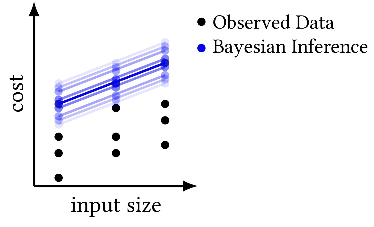
Figure 1 displays a schematic diagram of Bayesian resource analysis. We perform Bayesian inference to infer a posterior distribution of cost bounds (blue lines) from the runtime cost measurements (black dots).

To illustrate Bayesian resource analysis, consider the function split that was introduced earlier. Its resource-annotated type has the form $$ x : L^{q_0} (\mathtt{int}) \vdash \mathtt{split} \; x : L^{q_1} (\mathtt{int}) \times L^{q_2} (\mathtt{int}) $$ where the resource annotations \(q_0, q_1, q_2 \in \mathbb{R}_{\geq 0}\) are to be inferred by Bayesian inference.

Let a dataset \(\mathcal{D}\) of runtime cost measurements be $$ \mathcal{D} \coloneqq \{(x_i,(y_{i,1}, y_{i,2}),c_i) \mid 1 \leq i \leq n \} $$ where \(x_i\) is an input list, \((y_{i,1}, y_{i,2})\) is a pair of two output lists, and \(c_i\) is the cost of running \(\mathtt{split} \; x_i\).

The user constructs a probabilistic model \(p (\theta, D)\) based on whatever domain knowledge¹ they have. For example, a probabilistic model for split can be $$ \begin{aligned} q_0, q_1, q_2 & \sim \mathrm{Normal}_{[0, \infty)}(0, 5) \\ c_{i, \text{predict}} & = q_0 \lvert x_i \rvert - q_1 \lvert y_{i,1} \rvert - q_2 \lvert y_{i,2} \rvert & \qquad (i = 1, \ldots, n) \\ c_i & \sim \mathrm{Normal}_{[0, c_{i, \text{predict}}]}(c_{i, \text{predict}}, 2) & (i = 1, \ldots, n) \end{aligned} $$ The first line states that the resource annotations \(q_0, q_1, q_2\) follow a normal distribution truncated to the non-negative region. In the second line, the predicted costs \(c_{i, \text{predict}}\) are defined as \( q_1 \lvert v_i \rvert - q_2 \lvert y_{i,1} \rvert - q_3 \lvert y_{i,2} \rvert \), which is the difference between input and output potential. The third line states that the observed costs \(c_i\) from the dataset \(\mathcal{D}\) follow a normal distribution truncated to the interval \([0, c_{i, \text{predict}}]\). The distribution is truncated because the prediction of a worst-case cost bound must be larger than or equal to the observed cost.

Unsoundness

Data-driven analysis can infer a cost bound for any program \(P\), provided that it terminates. When we construct a dataset \(\mathcal{D}\) of the program \(P\)’s runtime cost measurements, the program must terminate on all inputs; otherwise, we will never finish collecting runtime cost measurements. Once we finish data collection, we statistically infer a polynomial cost bound from the dataset \(\mathcal{D}\). As the dataset \(\mathcal{D}\) is finite, for any degree \(d \geq 0\), we always have some degree-\(d\) polynomial bound \(\text{cost}_P\) that lies above all runtime cost measurements of \(\mathcal{D}\). Therefore, data-driven analysis always returns an inference result.

However, data-driven analysis lacks the soundness guarantee² of inference results. Data-driven analysis examines runtime cost data of the input program \(P\), rather than its source code. Consequently, data-driven analysis cannot reason about the theoretically worst-case behavior of the program \(P\), failing to provide a soundness guarantee.

For illustration, we ran Bayesian resource analysis on the median-of-medians-based linear-time selection algorithm. To collect cost measurements, we randomly generated input lists. Figure 2 plots the inferred posterior distribution of cost bounds. Black dots are runtime cost measurements. The light-blue shade is the 10-90th percentile range of the posterior distribution, and the blue line is the median cost bound. The red line is the true worst-case cost bound.

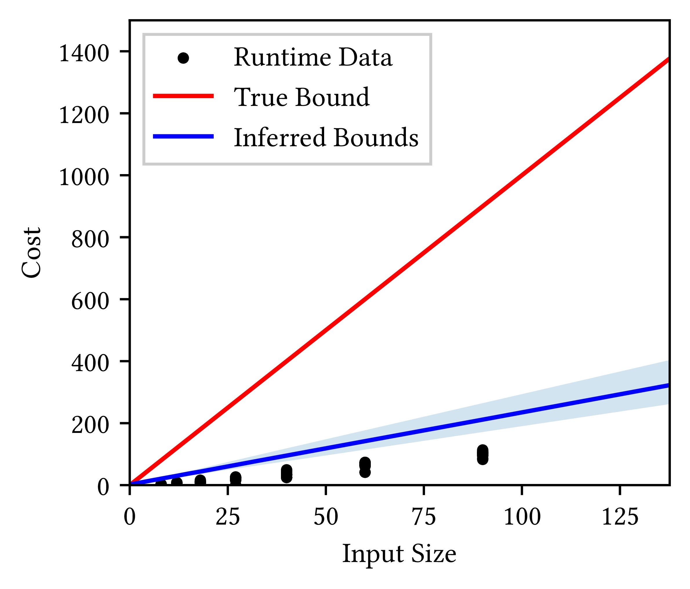
Although the inferred cost bounds (light-blue shade) all lie above the observed costs (black dots), they are unsound worst-case cost bounds since they lie below the true worst-case cost bound (red line). The true cost bound (red line) is significantly larger than observed costs (black dots) because, when inputs are randomly generated, the worst-case behavior of the selection algorithm rarely arises.

Certainly, we can fix this problem by adjusting the probabilistic model such that it adds more buffer on top of the maximum observed costs in the dataset \(\mathcal{D}\). However, it is difficult to tell a priori how much buffer we should add. On the other hand, static analysis is better suited for reasoning about the worst-case behavior than data-driven analysis. But if we perform static analysis on the entire source code of the linear-time selection algorithm, the analysis fails as described earlier. Can we perform static analysis on a fragment of the source code and data-driven analysis on the rest?

Hybrid Analysis

To overcome the limitations of purely static analysis (e.g., conventional AARA) and purely data-driven analysis (e.g., Bayesian resource analysis), we integrate them into a framework called hybrid AARA.

Hybrid AARA

First, a user indicates which part of the source code should be analyzed by data-driven analysis. For example, if we want expression e to be analyzed by data-driven analysis, we enclose e with the annotation statistics, resulting in statistics(e). The rest of the source code will be analyzed by static analysis. To construct a dataset \(\mathcal{D}\) of runtime cost measurements, we run the program \(P\) on many inputs (to \(P\)) and record the inputs, outputs, and costs of the expression e inside statistics(e). Here, the input to the expression e is its evaluation context (i.e., the values of free variables appearing in e) during the program \(P\)’s execution.

The data-driven analysis of the expression e incorporates its contextual information at runtime as the dataset \(\mathcal{D}\) captures this contextual information. For example, suppose statistics(e) appears inside the if-branch of a conditional expression if ... then ... else .... If the if-branch satisfies some invariant (e.g., inside the if-branch, variable x appearing inside e is even), then all measurements recorded in the dataset \(\mathcal{D}\) satisfy this invariant. Thus, data-driven analysis does not analyze the expression e in isolation from its context.

Next, we infer a cost bound in hybrid AARA. Given a program \(P\) containing statistics(e) for some expression e, we perform data-driven analysis on e and static analysis on the rest of the source code, and then combine their inference results. Just like we did for the cost-bound inference of conventional AARA, we assign variables to inputs and outputs throughout the source code of the program \(P\), where these variables stand for yet-to-be-inferred resource annotations. In hybrid AARA, however, we do not assign variables inside the expression e. That is, the expression e is treated as a black box whose source code is invisible. Let \(\theta_e\) be the set of resource annotations in the input and output of the expression statistics(e). Also, let \(\theta \supseteq \theta_e\) be a set of all variables in the program \(P\)’s entire source code.

A key challenge in hybrid AARA is the interface between conventional AARA and Bayesian resource analysis. Suppose conventional AARA generates a set \(C\) of linear constraints over the variables \(\theta\). Any solution to the linear constraints \(C\) is a valid cost bound. Conventional AARA optimizes the variables \(\theta\) subject to the linear constraints \(C\). This optimization problem is solved by an LP solver. On the other hand, Bayesian resource analysis infers a posterior distribution of the variables \(\theta_e \subseteq \theta\) by running a sampling-based Bayesian inference algorithm. Thus, conventional AARA and Bayesian resource analysis both involve the variables \(\theta_e\) in common, but they each use different algorithms for inference. How do we design their interface?

One idea is to restrict the state space of the sampling algorithm to the feasible region of the linear constraints \(C\). We first construct a probabilistic model over all variables \(\theta \supseteq \theta_e\), which represent resource annotations in the program \(P\)’s source code. We then run a sampling-based Bayesian inference algorithm over these variables, subject to the linear constraints \(C\). Thanks to the constraints \(C\), any cost bound drawn from the posterior distribution is a valid cost bound according to conventional AARA.

To implement hybrid AARA, we rely on recent advances in the literature of sampling algorithms. In 2021, a C++ library volesti started to support sampling from a user-specified probability distribution subject to arbitrary linear constraints. This is the first (and so far, only) tool that supports such sampling. Popular programming languages for Bayesian inference, such as Stan, only support box constraints (i.e., upper and lower bounds) on random variables, but not arbitrary linear constraints that may involve multiple variables.

Evaluation

We ran Hybrid AARA on the linear-time selection algorithm. Inside the selection algorithm’s source code, the code fragment partition x m, which partitions list x around the median of medians m, is analyzed by data-driven analysis. The rest of the source code is analyzed by static analysis. Figure 3 displays the inference results.

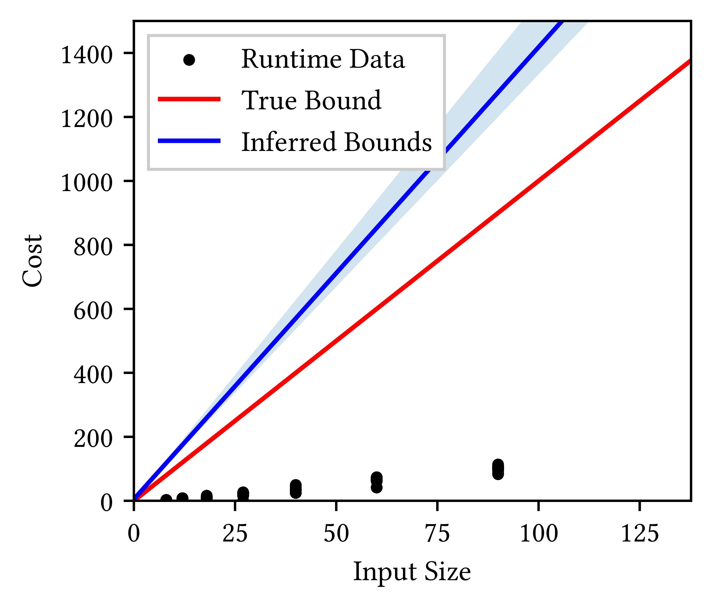
In Figure 3, the 10-90th percentile ranges (light-blue shade) of inferred cost bounds now contain or lie above the ground truth (red line). This is a significant improvement over Bayesian resource analysis (Figure 2), where the inferred cost bounds are below the true worst-case bounds.

More generally, we have evaluated hybrid AARA on a suite of seven benchmarks: MapAppend, Concat, InsertionSort2, QuickSort, QuickSelection, MedianOfMedians (this is the linear-time selection algorithm we have seen in this blog post), and ZAlgorithm. Conventional AARA fails in all benchmarks as they each contain a code fragment that cannot be analyzed statically by conventional AARA. Further, in all benchmarks, hybrid AARA infers cost bounds closer to the true worst-case cost bounds than purely data-driven resource analysis. Thus, our evaluation demonstrates the benefits of hybrid resource analysis: hybrid analysis infers more accurate worst-case cost bounds than purely data-driven analysis, while overcoming the incompleteness of purely static analysis. The details of the evaluation can be found in out paper Robust Resource Bounds with Static Analysis and Bayesian Inference.

Conclusion

Hybrid resource analysis combines purely static analysis, which offers soundness guarantees of worst-case cost bounds but is incomplete, and purely data-driven analysis, which is not sound but can infer a cost bound for any program. By combining these two complementary analysis techniques, hybrid resource analysis successfully infers cost bounds that neither purely static analysis nor purely data-driven analysis can infer. This is demonstrated by the experiment results of the linear-time selection algorithm.

Hybrid AARA has a limitation that its data-driven analysis only infers resource annotations, but not other quantities (e.g., depth of recursion). As a result, hybrid AARA cannot handle some programs such as bubble sort. In bubble sort, conventional AARA cannot infer the number of recursive calls, but it can still correctly infer a cost bound of each recursive call. Therefore, ideally, we would like to infer (i) the number of recursive calls by data-driven analysis and (ii) the cost of each recursive call by conventional AARA. This requires a different hybrid analysis technique from hybrid AARA presented in this blog post, and we plan to investigate it as future work.

Acknowledgement: hybrid AARA is joint work with Feras Saad and Jan Hoffmann. Our paper Robust Resource Bounds with Static Analysis and Bayesian Inference is currently under review, and hopefully we can share it soon.

Further reading: the original paper on AARA targets linear cost bounds. Subsequently, AARA has been extended to univariate polynomial cost bounds and multivariate polynomial cost bounds. Resource-aware ML is an implementation for AARA for analyzing OCaml programs. Papers on data-driven resource analysis include the trend profiler, algorithmic profiler, and input-sensitive profiler. They are all concerned with average-case cost bounds, rather than worst-case cost bounds as in this blog post. Also, these papers all use optimization instead of Bayesian inference.