
Measuring and Exploiting Network Usable Information
In large cloud service providers such as AWS, the customer provides an attributed graph and would like to perform tasks such as recommendations (i.e., link prediction in a graph) using message-passing methods within restricted budgets. An attributed graph consists of both the graph structure and the node features. As one of the message-passing methods, Graph Neural Networks (GNNs) are commonly used for graph tasks by propagating node features through the graph structure. However, it is possible that not all the information in the provided graph is usable for solving the task. Training a GNN would thus be a waste of time and resources for the customer. Therefore, we aim to answer two questions:
- Given a graph with node features, how can we tell whether utilizing both graph structure and node features will yield better performance than utilizing either of them separately?
- How can we know what information in the graph (if any) is usable to solve the tasks, namely, node classification and link prediction?
Our goal is to design a metric for measuring how informative the graph structure and node features are for the task at hand, which we call network usable information (NUI).
In this blog post, we introduce how to measure the information in the graph, and to exploit it for solving the graph tasks. This blog post is based on our research paper, “NetInfoF Framework: Measuring and Exploiting Network Usable Information” [1], presented at ICLR 2024.
What is an attributed graph?

A graph is a data structure that includes nodes and edges, representing the connections between nodes. An attributed graph indicates that each node in the graph has a set of features. For example, Figure 1 shows the attributed graph for a social network. The nodes represent the users, illustrated as circles with university acronyms. The edges indicate whether two users are friends, illustrated as black lines connecting circles. A node might also contain additional information:
- Node ID : illustrated as a thumbnail image of the user along with the user’s text name.
- Node attributes/features : represent whether the user is located in the US and whether the user likes to bike, illustrated as a table.
- Node label : signifies the user’s university, categorized into two groups represented by blue and red colors with acronyms: Carnegie Mellon University (CMU) or National Chiao Tung University (NCTU).
In fact, node labels are similar to node features, but they often contain missing values, which we are interested in predicting.
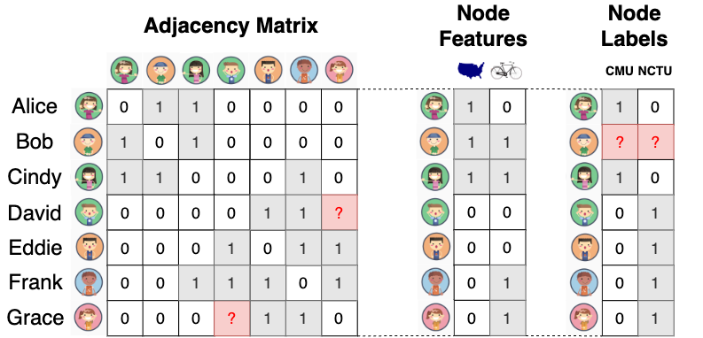
In Figure 2, the graph structure can be represented by an adjacency matrix, where 1 denotes the presence of an edge between two nodes, and 0 denotes no edge. The node features are also represented by a matrix, where each feature is binary in the example, but it can also be continuous. The node labels are represented by a matrix with one-hot encoding of the class label.
What are the common graph tasks?
We consider the two common graph tasks:
-
Node Classification
- Goal: Classify the unlabeled nodes, while some labeled nodes are given.
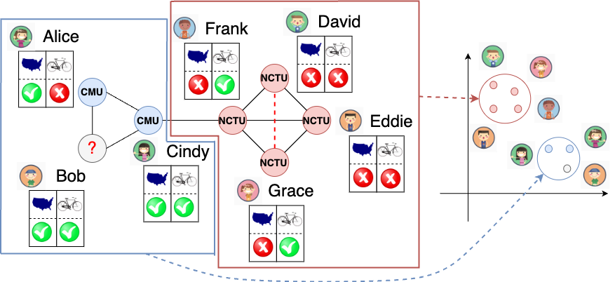
- Example: Given a social network with features, can we guess which university Bob goes to, i.e., the label of the gray node in Figure 1?
-
Link Prediction
- Goal: Predict the potential additional edges in the graph.
- Example: Given a social network with features, can we guess whether David and Grace could become friends, i.e., the potential additional red-dash line in Figure 1?
What are message-passing methods?
Message-passing methods utilize the graph structure to propagate information from the neighbors of a node to the node itself. Known as sum-product message-passing, belief propagation methods [2, 3] directly perform inference on the graph through several propagation iterations. Although they are fast and effective because they require neither parameters nor training, belief propagation methods are mainly designed to solve node classification problems based solely on the graph structure and usually do not consider node features.
Another variety of message-passing methods, Graph Neural Networks (GNNs) [4], are a class of deep learning models. They are commonly used to generate low-dimensional embeddings of nodes to perform graph tasks by learning end-to-end with a training objective. As shown in Figure 3, the nodes that are better connected in the graph are expected to have closer embeddings in the low-dimensional space.
Some studies remove the non-linear functions in GNNs, and still achieve good performance, which we call linear GNNs [5, 6]. One of the many advantages of linear GNNs is that their node embeddings are available prior to model training. A comprehensive study on linear GNNs can be found in [6].
Measuring NUI: Would a message-passing method work in a given setting?

Given an attributed graph, how can we measure the network usable information (NUI)? The message-passing method may not work well in the following two conditions:
- No network effects: the graph structure is not useful to solve the graph task. In Figure 4(a), since every labeled node has one blue and one red neighbor, we cannot infer the label for Bob by examining its neighbors.
- Useless node features: the node features are not useful to solve the graph task. In Figure 4(b), we can see that whether a user likes to bike is not correlated with the user’s university.
If either of these two extreme conditions applies, a message-passing method is likely to fail in inferring the unknown node label, i.e., Bob’s university. However, it is very likely that the graph information has varying levels of usefulness, ranging between completely useful and completely useless. For example, in Figure 2, only 1 out of 2 node features is useful: the node feature ‘located in the US’ is useful, while the node feature ‘likes to bike’ is not.
We focus on analyzing whether GNNs will perform well in a given setting, which is an important problem in the industry. The reason is that, for large cloud service providers, the customer provides them with an attributed graph and requests them to solve the graph task (e.g., recommendation) using GNNs within restricted budgets. However, if the given graph lacks network usable information (NUI), the resources spent on training GNNs will be wasted. Therefore, our method serves as a preliminary tool to determine whether resources should be allocated for training expensive deep models.
A straightforward way is to analyze the node embedding of the given graph generated by GNNs, but this is only available after training, which is expensive and time-consuming. For this reason, we propose to analyze the derived node embedding in linear GNNs, which can be precomputed before model training. More specifically, we derive three types of node embedding that can comprehensively represent the information of the given graph, namely:
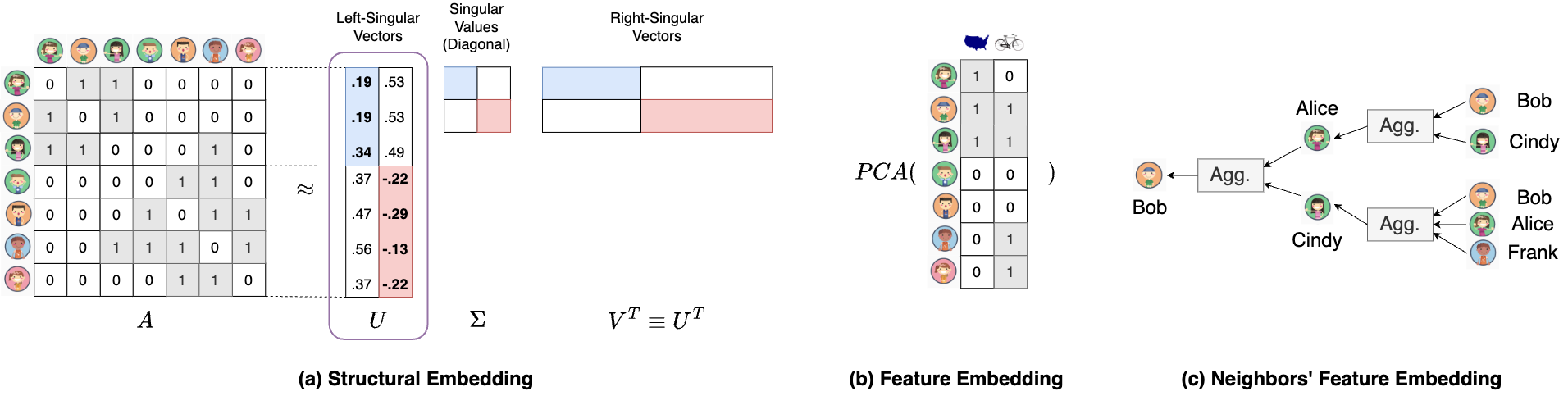
- Structural embedding (): for the information of the graph structure. It is extracted by decomposing the adjacency matrix with singular value decomposition (SVD). Intuitively, the left singular vectors U give the information of the node community. For example, in Figure 5(a), U identifies that the first three users belong to the blue community, while the last four belong to the red community. This is useful when the node features are not useful to solve the graph task.
- Feature embedding (): for the information of the node features. It consists of the original node features after dimensionality reduction. As shown in Figure 5(b), Principal Component Analysis (PCA) [7] is used as the dimensionality reduction technique. This is useful when there are no network effects, i.e. the graph structure is not useful to solve the graph task.
- Neighbors’ feature embedding (): for the information of the features aggregated from the neighbors. As shown in Figure 5(c), the messages are passed and aggregated from the neighbors for two steps. The intuition is that, in addition to the information from the user, the user’s neighbors also provide useful information to the task. Leveraging their information leads to better performance on the graph task. This is useful when both the graph structure and the node features are useful to solve the graph task.
Once we have the embedding that can represent the information of the nodes of the graph, we propose NetInfoF_Score, and link the metrics of graph information and task performance with the following proposed theorem:
Definition 1 (NetInfoF_Score of given ). Given two discrete random variables and , NetInfoF_Score of given is defined as: where denotes the conditional entropy [8].
Theorem 1 (NetInfoF_Score). Given two discrete random variables and , NetInfoF_Score of given lower-bounds the accuracy: where is the joint probability of and .
The proof is in [1]. The intuition behind this theorem is that the conditional entropy of (e.g. labels) given (e.g. “like biking”), is a strong indicator of how good of a predictor is, to guess the target . It provides an advantage to NetInfoF_Score by giving it an intuitive interpretation, which is the lower-bound of the accuracy. When there is little usable information for the task, the value of NetInfoF_Score is close to random guessing.

In Figure 6, each point represents the accuracy and NetInfoF_Score obtained by solving graph tasks using one type of node embedding. We find that NetInfoF_Score lower-bounds the accuracy of the given graph task, as expected. If an embedding has no usable information to solve the given task, NetInfoF_Score gives a score close to random guessing (see lower left corner in Figure 6). The details of the experiment can be found in [1].
Exploiting NUI: How to solve graph tasks?
In this blog, we focus on explaining how to solve node classification. How to solve link prediction is more complicated, and the details can be found in [1].
To solve node classification, we concatenate different types of embedding, and the input of the classifier is as follows: where is concatenation, is the structural embedding, is the feature embedding, and is the neighbors’ feature embedding. Among all the choices, we use logistic regression as the node classifier, as it is fast and interpretable.
How well does our proposed method perform?
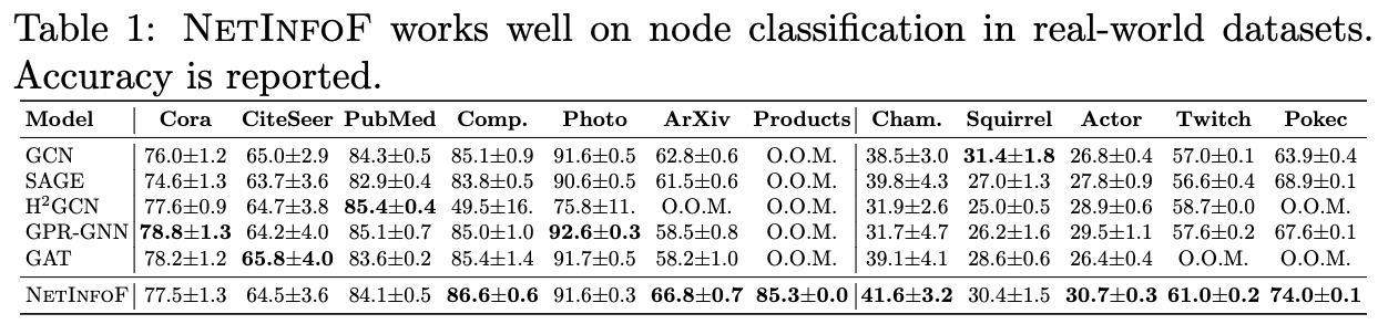
As shown in Table 1, applied on 12 real-world graphs, NetInfoF outperforms GNN baselines in 7 out of 12 datasets on node classification.
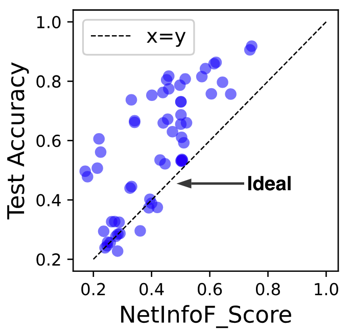
In Figure 7, NetInfoF_Score is highly correlated with test performance on node classification. This indicates that NetInfoF_Score is a reliable measure for deciding whether to use a GNN on the given graph or not in a short time, without any model training. Noting that although our theorem proves that NetInfoF_Score is a lower bound on training accuracy, it is possible for testing accuracy to be lower than the NetInfoF_Score (blue points below 45 degree line in Figure 7).
Conclusion
In this blog post we investigate the problem of predicting whether a message-passing method would work well on a given graph. To solve this problem, we introduce our approach called NetInfoF to measure and exploit the network usable information (NUI). Applied on real-world graphs, NetInfoF not only correctly measures NUI with NetInfoF_Score, but also outperforms other baselines 7 out of 12 times on node classification.
Please find more details in our paper [1].
References
[1] Lee, M. C., Yu, H., Zhang, J., Ioannidis, V. N., Song, X., Adeshina, S., … & Faloutsos, C. NetInfoF Framework: Measuring and Exploiting Network Usable Information. International Conference on Learning Representations (ICLR), 2024.
[2] Koutra, D., Ke, T. Y., Kang, U., Chau, D. H., Pao, H. K. K., & Faloutsos, C. Unifying guilt-by-association approaches: Theorems and fast algorithms. Machine Learning and Knowledge Discovery in Databases: European Conference (ECML PKDD), 2011
[3] Günnemann, W. G. S., Koutra, D., & Faloutsos, C. Linearized and Single-Pass Belief Propagation. VLDB Endowment, 2015.
[4] Kipf, T. N., & Welling, M. Semi-Supervised Classification with Graph Convolutional Networks. International Conference on Learning Representations (ICLR), 2017.
[5] Wu, F., Souza, A., Zhang, T., Fifty, C., Yu, T., & Weinberger, K. Simplifying Graph Convolutional Networks. PMLR International Conference on Machine Learning (ICML), 2019.
[6] Yoo, J., Lee, M. C., Shekhar, S., & Faloutsos, C. Less is More: SlimG for Accurate, Robust, and Interpretable Graph Mining. ACM SIGKDD Conference on Knowledge Discovery and Data Mining (KDD), 2023.
[7] Principal component analysis. In Wikipedia. https://en.wikipedia.org/wiki/Principal_component_analysis , 2024.
[8] Conditional entropy. In Wikipedia. https://en.wikipedia.org/wiki/Conditional_entropy , 2024.