Word Embedding Demo: Tutorial

Semantic Feature Space

Consider the words "man", "woman", "boy", and "girl". Two of them refer to males, and two to females. Also, two of them refer to adults, and two to children. We can plot these worlds as points on a graph where the x axis axis represents gender and the y axis represents age:

Gender and age are called semantic features: they represent part of the meaning of each word. If we associate a numerical scale with each feature, then we can assign coordinates to each word:

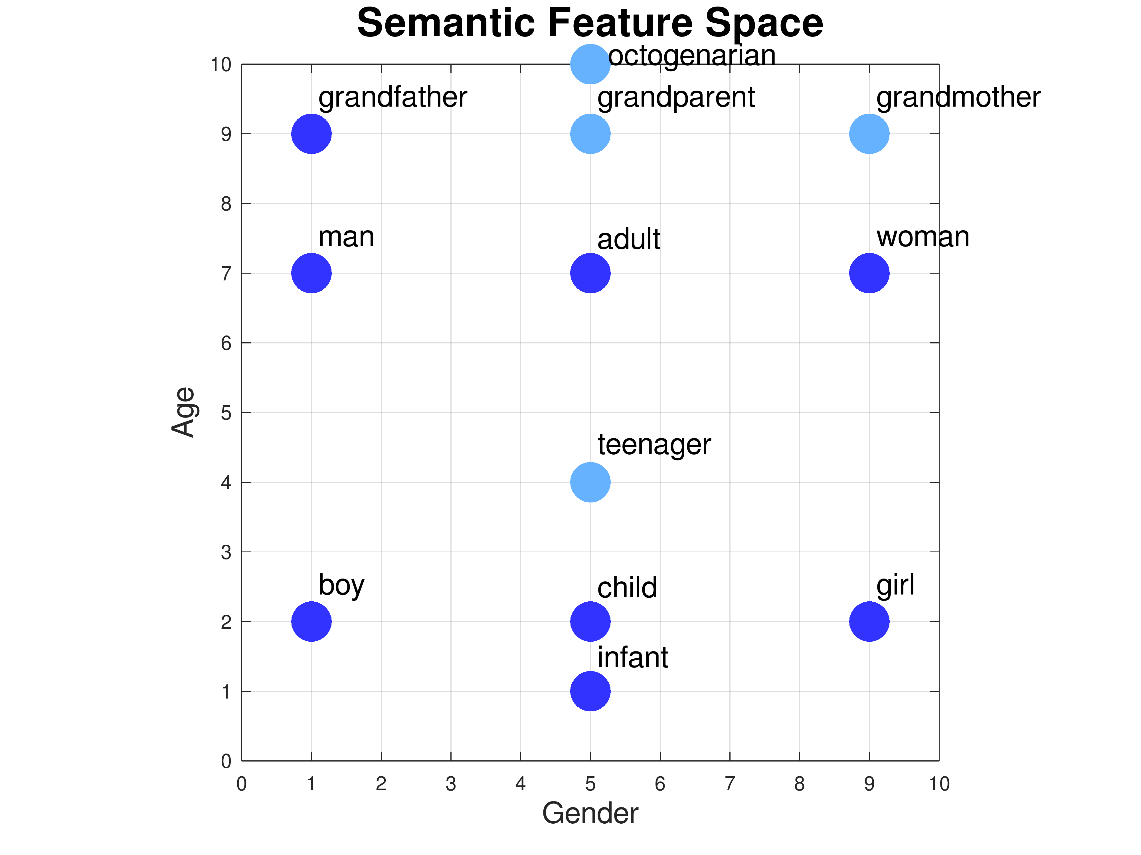
We can add new words to the plot based on their meanings. For example, where should the words "adult" and "child" go? How about "infant"? Or "grandfather"?

Word Coordinates Gender Age grandfather [ 1, 9 ] man [ 1, 7 ] adult [ 5, 7 ] woman [ 9, 7 ] boy [ 1, 2 ] child [ 5, 2 ] girl [ 9, 2 ] infant [ 5, 1 ]

Exercise: how would you represent the words "grandmother", "grandparent", "teenager", and "octogenarian"?

Answer: The gender coordinates are obvious. We can extrapolate the age coordinates based on the values for the words we've already defined:

Word Coordinates Gender Age grandmother [ 9, 9 ] grandparent [ 5, 9 ] octogenarian [ 5, 10 ] teenager [ 5, 4 ]

Now let's consider the words "king", "queen", "prince", and "princess". They have the same gender and age attibutes as "man", "woman", "boy', and "girl". But they don't mean the same thing. In order to distinguish "man" from "king", "woman" from "queen", and so on, we need to introduce a new semantic feature in which they differ. Let's call it "royalty". Now we have to plot the points in a 3-dimensional space:

Word Coordinates Gender Age Royalty man [ 1, 7, 1 ] woman [ 9, 7, 1 ] boy [ 1, 2, 1 ] girl [ 9, 2, 1 ] king [ 1, 8, 8 ] queen [ 9, 7, 8 ] prince [ 1, 2, 8 ] princess [ 9, 2, 8 ]

Uses of Semantic Feature Vectors

Semantic distance is a way to measure relatedness of words. Google's Semantris is a game that uses feature vector representations to determine which words or phrases are related to which other words. It's worth exploring.

An even more interesting thing we can do with semantic feature vectors is solve word analogy problems.

Analogies By Vector Arithmetic

We can also represent word analogies graphically. For the relationship of "man" to "king" we draw an arrow from "man" to "king". Next we copy this arrow, keeping the same direction and length, but now starting from "woman". Then we see where the arrow points and look for the closest word:

Word Embeddings

Instead we can let the computer create the feature space for us by supplying a machine learning algorithm with a large amount of text, such as all of Wikipedia, or a huge collection of news articles. The algorithm discovers statistical relationships between words by looking at what other words they co-occur with. It uses this information to create word representations in a semantic feature space of its own design. These representations are called word embeddings. A typical embedding might use a 300 dimensional space, so each word would be represented by 300 numbers. The figure below shows the embedding vectors for six words in our demo, which uses a 300-dimensional embedding. "Uncle", "boy", and "he" are male words, while "aunt", "girl", and "she" are female words. Each word is represented by 300 numbers with values between -0.2 and +0.2. Component number 126 is shown magnified to the left. As you can see, component 126 appears to correlate with gender: it has slightly positive values (tan/orange) for the male words and slightly negative values (blue/gray) for the female words.

This rich semantic space supports many kinds of analogies, such as pluralization ("hand" is to "hands" as "foot" is to "feet"), past tense ("sing is to sang as eat is to ate"), comparisons ("big" is to "small" as "fast" is to "slow"), and even mapping countries to their capitals ("France" is to "Paris" as "England" is to "London").

The most significant application of word embeddings is to encode words for use as input to complex neural networks that try to understand the meanings of entire sentences, or even paragraphs. One such class of networks are called transformer neural networks. Two famous transformer networks are BERT from Google and GPT3 from OpenAI. BERT now handles many Google searches.

Measuring Euclidean Distance

We've been drawing words as points in a semantic space, and we've also referred to these points as vectors. In mathematics, a vector is drawn as an arrow, and it consists of a length and a direction. Words can be drawn as arrows that begin at the origin and end at the point. So the word "child" can be drawn as an arrow from the origin [0, 0] to the point [5, 2]. Here are all the words in our 2D semantic space drawn as vectors:

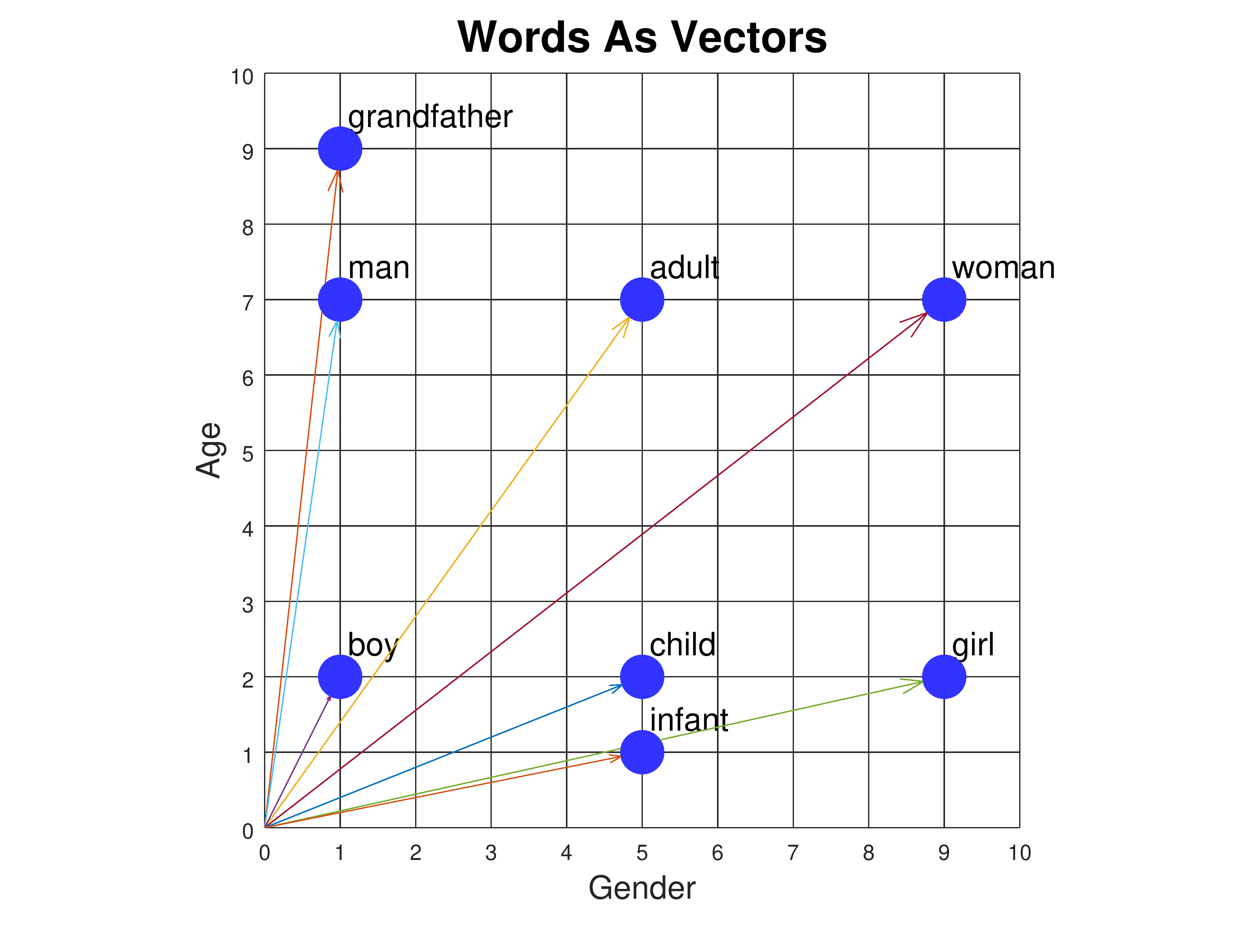
We can compare two words by drawing a vector from one to the other and measuring its length. The vector from "boy" to "infant" can be computed by starting with "infant" [5,1] and subtracting "boy" [1,2], giving the vector [4, -1]. The length of a vector [x, y] is given by the formula sqrt(x² + y²), where sqrt is the square root function. So the vector from "boy" to "infant" has a length of sqrt(17), or about 4.12. This is the Euclidean distance between the two words. Here are the vectors from "boy" to all the other words, and their lengths:

Distance from "boy" grandfather 7 man 5 adult 6.4031 woman 9.4340 boy 0 child 4 girl 8 infant 4.1231

You can see that the closest word to "boy" is "child", but "infant" is only a little bit further away.

The same Euclidean distance formula works in higher dimensions too. The length of a 3D vector [x, y, z] is sqrt(x² + y² + z²).

Euclidean distance is a perfectly reasonable distance measure, but it's not the preferred distance measure for word embeddings. Instead we use something called the dot product. It's actually a similarity measure rather than a distance measure. Larger values mean words are more similar.

Measuring Similarity With Dot Product

Original Word Vectors grandfather [ 1, 9 ] man [ 1, 7 ] adult [ 5, 7 ] woman [ 9, 7 ] boy [ 1, 2 ] child [ 5, 2 ] girl [ 9, 2 ] infant [ 5, 1 ]

In the above diagram, the angle between "boy" (maroon vector) and "adult" (yellow vector) is small, while the angle between "boy" and "child" (blue vector) is larger. But clearly "boy" is closer to "child" than to "adult", since "boy" differs only modestly from "child" in the gender coordinate, while it differs from "adult" in both the gender and age coordinates. The problem is that all our vectors originate at the origin. To correct the problem and make angle a useful measure of similarity, we need the vectors to originate at the center of all the points. So let's move the points so that their center is at the origin. We can do this by taking the mean (average) of all the points and subtracting that value from every point. This means that for every feature, some words will have negative feature values while others will have positive feature values, so that their average is zero. Shifting the coordinates this way has no effect on the Euclidean distance measure because all points are shifted by the same amount. But it dramatically affects the dot product. The result looks like this:

Zero-Mean 2D Vectors grandfather [ -3.500, 4.375 ] man [ -3.500, 2.375 ] adult [ 0.500, 2.375 ] woman [ 4.500, 2.375 ] boy [ -3.500, -2.625 ] child [ 0.500, -2.625 ] girl [ 4.500, -2.625 ] infant [ 0.500, -3.625 ]

Now the angle between the "boy" and "child" vectors is much smaller than the angle between "boy" and "adult", as it should be because "boy" and "child" only differ by 4 in their gender coordinates, whereas "boy" and "adult" differ both by 4 in their gender coordinates and by 5 in their age coordinates. But there is still an issue. The dot product of two vectors is not exactly the cosine of the angle θ between them; it's proportional to the cosine. Given two vectors u and v, the exact value of u·v is cos(θ)·||u||·||v||, where ||u|| is the length of the vector u, i.e., its Euclidean distance from the origin. If we want the dot product to exactly equal the cosine, we need to normalize the vectors so that they have length 1. We do this by dividing the coordinates of each vector by the length of the vector, i.e., given a vector u = [x, y] with length ||u|| = sqrt(x² + y²), we can construct a unit vector pointing in the same direction but with a length of 1 as u/||u|| or [x/||u||, y/||u||].

Here is what the points look like when we convert them to unit vectors, so they all lie on a circle of radius 1:

Zero-Mean 2D Unit Vectors grandfather [ -0.6247, 0.7809 ] man [ -0.8275, 0.5615 ] adult [ 0.2060, 0.9785 ] woman [ 0.8844, 0.4668 ] boy [ -0.8000, -0.6000 ] child [ 0.1871, -0.9823 ] girl [ 0.8638, -0.5039 ] infant [ 0.1366, -0.9906 ]

The dot product and Euclidean distance measures produce results that are similar but not identical. For example, based on Euclidean distance, "boy" is slightly closer to "child" than to "infant", but looking at the unit vectors in the figure above, the angle between "boy" and "infant" is slightly less than the angle between "boy" and "child".

The word embeddings used in this demo, and by real AI systems, are unit vectors with zero mean, just like the points above. The same normalization technique applies to higher dimensional vectors, e.g., for three-dimensional semantic vectors, the points lie on the surface of a unit sphere (a sphere with radius 1), as shown below:

Zero-Mean 3D Unit Vectors Gender Age Royalty grandfather [ -0.5426, 0.6412, -0.5426 ] man [ -0.7191, 0.4576, -0.5230 ] woman [ 0.7741, 0.4168, -0.4764 ] boy [ -0.6971, -0.5070, -0.5070 ] girl [ 0.7543, -0.4642, -0.4642 ] king [ -0.5570, 0.5064, 0.6583 ] monarch [ 0.0676, 0.4730, 0.8785 ] queen [ 0.6608, 0.3558, 0.6608 ] prince [ -0.5846, -0.4252, 0.6909 ] princess [ 0.6484, -0.3990, 0.6484 ] child [ 0.0733, -0.5866, -0.8066 ] infant [ 0.0642, -0.7057, -0.7057 ]

How Word Embeddings Are Created

Step 1: Assemble a text corpus. We might choose Wikipedia articles, or a collection of news stories, or the complete works of Shakespeare. The corpus determines the vocabulary we have to work with and the co-occurrence statistics of words, since different writing styles will use words differently.

Step 2: Choose a vocabulary size M. A large corpus could contain one million distinct words if we include person names and place names. Many of those words will occur infrequently. To keep the embedding task manageable we might decide to keep only the highest frequency words, e.g., we might choose the 50,000 words that occur most frequently in the corpus. Filtering out the lowest-frequency words also eliminates typos, e.g., "graet" should probably have been "great", "grate", or "greet". At this stage we also need to decide how to handle punctuation, contractions, subscripts and superscripts, special characters such as Greek letters or trademark symbols, and alternative capitalizations.

Step 3: Choose a context window size C. If we use a context window of size C=2 we will look at five-word chunks. That is, for each word in the corpus we will treat the 2 words to the left of it and the 2 words to the right of it as its context.

Step 4: Assemble a co-occurrence dictionary. By proceeding one word at a time through the corpus and looking C words back and C words ahead, we can determine, for every target word, which words occur in its context. For example, with C=2, given the text "Thou shalt not make a machine in the likeness of a human mind", the co-occurrence dictionary would look like this:

Notice that the word "a" occurs twice in the corpus. Its contexts are combined in the dictionary. In practice the corpus would be much larger than this, with every word appearing multiple times, making for a much richer context.

Step 5: Choose an embedding size N so that each word will be represented by a list of N numbers. A typical value for N is 300, although small embeddings might use only 100 numbers per word, while large ones could use 700 or more. Larger values of N can encode more information, but the embedding takes longer to compute and more memory to store.

Step 6: Make two tables each containing M rows and N columns. Each row represents a word. For example, if we have a 50,000 word vocabulary and are constructing 300-element embeddings, the table would be of size 50,000 × 300. One table, E, is for the target words we're trying to embed. The second table, U, is for words when they are used as context words. Initialize both tables with small random numbers.

Step 7: This is the training process. Slide a window of size 2C+1 over the entire training corpus, shifting it by one word each time. For each target word t in the middle slot of the window, look up its vector e in the embedding table E. For each context word u occurring in some other slot of the window, look up its vector u in the context table U. Compute the dot product e·u and run the result through a non-linear squashing function (called the "sigmoid" or "logistic" function) that produces an output value between 0 and 1. If the output is less than 1, make a tiny adjustment to the vectors e and u using a technique called gradient descent learning; this technique is also used to train neural networks. Repeat the process for all the context words. These are the positive examples. We also need some negative examples. Choose 5 to 10 vocabulary words at random that our context dictionary indicates never appear in the context of the target word. Apply the same procedure as above, except now we want the value of the squashed dot product to be 0 rather than 1. Make tiny adjustments to the embedding and context vectors accordingly. We repeat this process, making a pass through the entire corpus, between 3 and 50 times.

Step 8: The embedding table E now contains the desired embeddings. The context table U can be discarded.

Additional Resources

• The Illustrated Word2Vec, by Jay Alammar.
• Interactive Visualizations of Word Embeddings for K-12 Students, by Saptarashmi Bandyopadhyay, Jason Xu, Neel Pawar, and David Touretzky. EAAI-22 (Educational Advances in Artificial Intelligence), February 26-27, 2022.
• TensorFlow word embeddings.
• Google's Semantris game, which uses word embeddings.
• GitHub repository for this WordEmbeddingDemo.