FMRI modeling
In this tutorial we will explore tools for analyzing functional brain imaging data, namely fMRI, however these methods can be applied to other types of neuroimaging data with the proper considerations.
Controlled experiments
In a typical fMRI experiment contains a small number of conditions. For example "nouns" and "verbs". Examples from each condition are shown to the subjects. This can be done either in multiple ways (see LINK).
Design matrix
One can build a design matrix of the experiment, indicating what stimulus was seen at every point in time.

Image adapted from here (fig 4).
Remember than fMRI measures a change in the blood oxygen levels, which is a delayed response after neural activity occurs. This is called the hemodynamic response. It peaks after a latency of about 6-8s after stimulus onset. There is evidence that the hemodynamic response is different in different parts of the brain (see LINK), but the usual approach is to assume a fixed shape for the entire brain. The exact parameters for shape of the response might vary, however, this is a typical shape of how it ends up being modeled:

The design matrix is convolved with this hypothetical hemodynamic response. The new design matrix is not similar to the following. It incorporates the delay of the hemodynamic response:

Image adapted from here (fig 4).
Generalized Linear Models
The typical approach to the analyzing fMRI data is to build a general linear model.
For example:
\begin{align} y_i = \beta_0 + x_{i,1}\beta_1 + x_{i,2}\beta_2 + x_{i,3}\beta_3 = X_i \beta \end{align}$y_i$ is the activity in one voxel. $X_i$ is a 4-dimentional vector (including an intercept term) and $\beta$ is a vector of parameters indicating the response of the voxels to the different conditions. Typically those conditions occur one at a time. The ANOVA is also a type of GLM.
Toolboxes
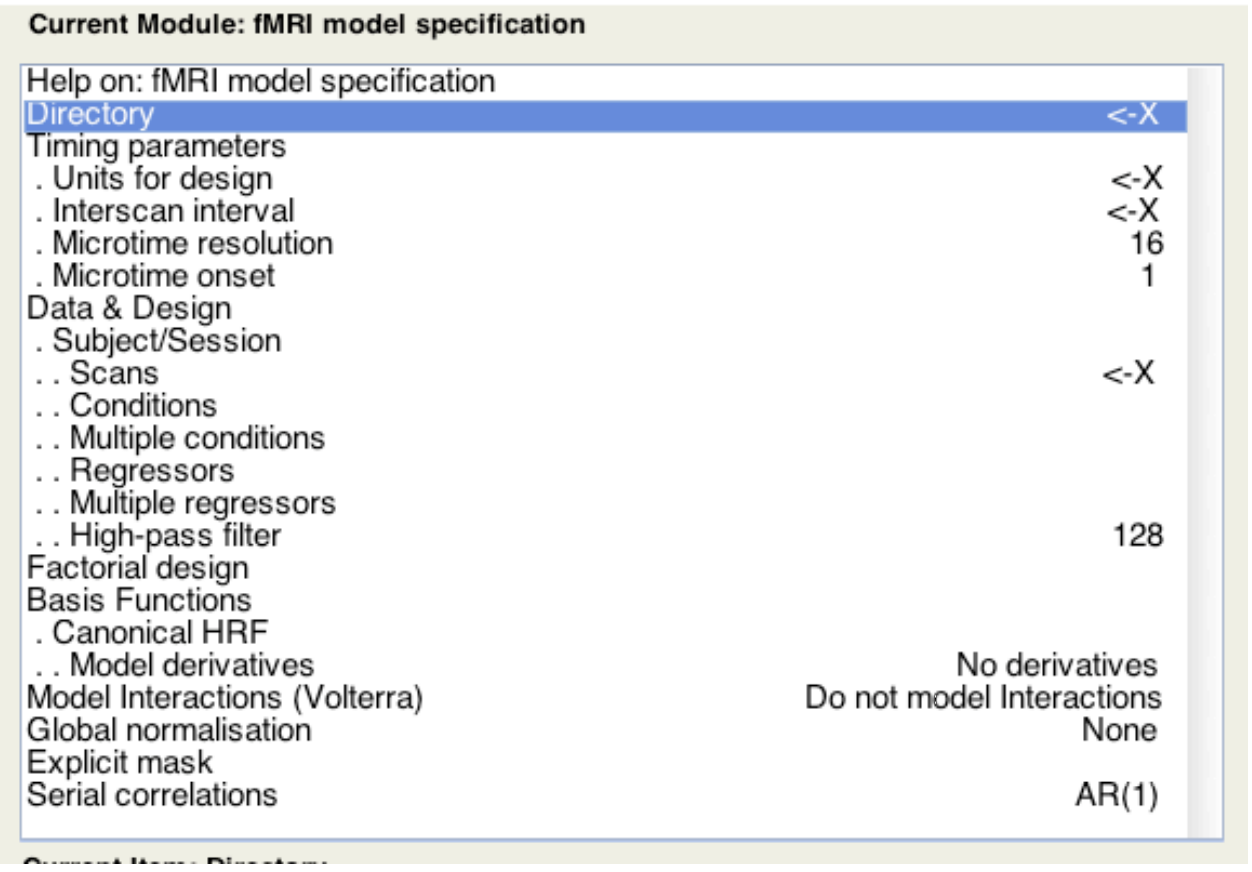
Many toolbox exist to run these analyses. For example in spm8, one can enter the occurence of all conditions:

SPM automatically builds the design matrix, and learn the GLM model. (One can also add other variables (such as motion, breathing and heart rate) into the regression. )
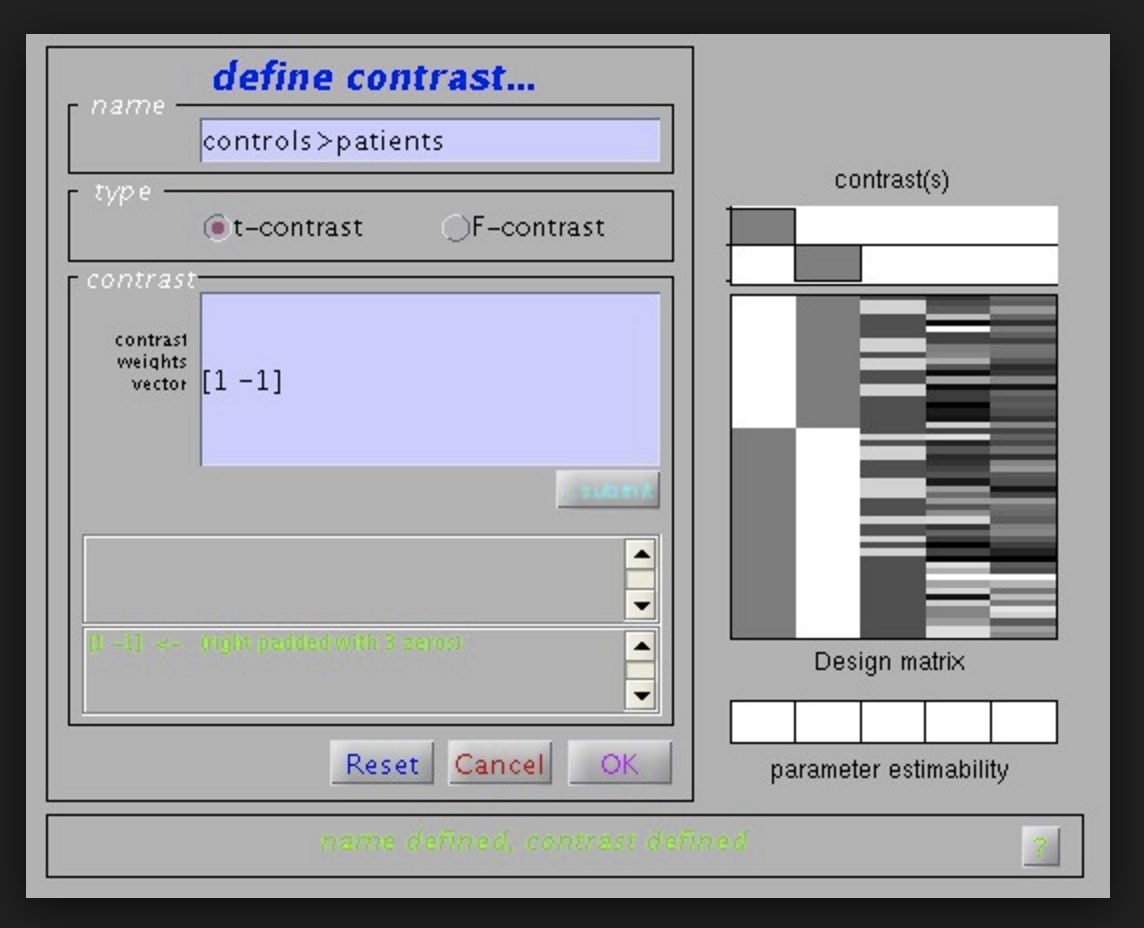
After the weights are learned the spm software will perform a test on them. For example we might specify a test to see where in the brain is condition A associated with an increase in activity? Or where does condition A increase brain activity more than B?
SPM will perform a T-test in this case such as in :

If we have more than one contrast we are looking at, SPM8 also allows us to perform an F-test.
However this is a computational neuroscience school, and therefore we will learn to perform our own analyses of data.
Brain Decoding
Instead of fitting the above function on a voxel by voxel basis, and seeing which voxels are different, there is a recent trend in using brain decoding. In brain decoding we look at multiple voxels at a time, from a region of the brain or the entire brain. We have activity $Y_i$ of a region or the entire brain. $Y_i$ can belong to condition A or B that we have to guess.
This relies on learning a classifier. A classifier is learned on training data, and it is very important not to test the classifier on any data that was used to learn the classifier or make any decision about its parameters.
The classifier sees multiple instances of condition A and condition B in training and determines their significant features. When faced with a new instance $Y_i$ as its input, it outputs a label A or B.
Common classifier that have been used with fMRI data are Linear Discriminant Analysis (LDA), support vector machines (SVM), Logistic Regression or Guassian Naive Bayes.
Complex Stimuli
However, the controlled experiment approach does not allow us to look at complex stimuli. What if we are interested in the variety of meanings that language can have? It will take an extremely long time to test everything single property one by one.
Another approach to neuroimaging is therefore to image the brain activity while the subject sees a large number of different stimuli that vary along multiple dimensions. The idea is to cover the space of variability so that the contribution of each feature of the stimulus can be recovered from the data.
%matplotlib inline
from matplotlib.pyplot import figure, cm
import matplotlib.pyplot as plt
from cortex_light.volume import mosaic
import numpy as np
import scipy.stats as stats
# this package allows us to work with matlab data
import scipy.io as sio

# here we load the variables in data_S1.mat as a dictionary called all_data
all_data = sio.loadmat('data/data_S1.mat')

# let's just start by making each voxel have mean 0 and variance 1, the function zscore does that:
data = stats.zscore(all_data['data'])
# data is N x nVoxels
print "We have {0} words, and for each word, we have an image with {1} voxels.".format(data.shape[0],data.shape[1])

# colToCoord is a nVoxels x 3 matrix, each row has the 3D coordinates of the ith voxel in the ith column of data
colToCoord = all_data['colToCoord']

dim = all_data['dim'][0]
print "\nThe 3D space has dimensions {}\n".format(dim)

words = [s[0][0] for s in all_data['words']]
print "Here are the stimulus words:\n"
print " - ".join(words)
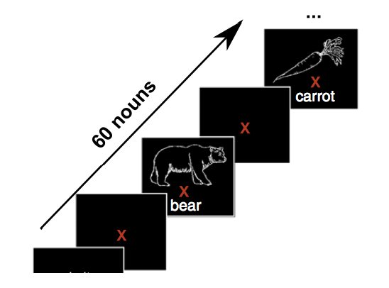
The experiment actually consist in subjects looking at words/line drawings that are presented in isolation:

We will use a function from the [pycortex package] (https://github.com/gallantlab/pycortex) to plot fMRI activity. This is a very powerful python package for the diplay of brain activity that is freely available.
In the below cell we sample some random data and see how the plotting function works, it just images a 3D volume.
random_sample = np.random.random_sample([16,64,64])
f = figure(figsize=(15,5))
h = mosaic(random_sample)
print "example of random data"
def make_3D_brain(data_row,colToCoord):
    brain = np.zeros(dim)+data_row.min() # makes background dark
    for i in range(colToCoord.shape[0]):
        row = colToCoord[i]
        brain[row[0]][row[1]][row[2]]= data_row[i]
    brain = np.transpose(brain,[2,1,0])
    return brain

f = figure(figsize=(15,5))

word_num = 0 # change the word number
brain_image = make_3D_brain(data[word_num],colToCoord) # takes a row of data and makes it in 3D
h = mosaic(brain_image) # can try with different color map: e.g. h = mosaic(image , cmap= cm.hot)
plt.title(words[word_num],size=30)
How can we represent the activity for items that do not belong into clear conditions? We see each word only once! However the stimuli are not completely independent, as they share some features.
Try changing feature_i below. Try to see the different features, as well as the features 218-229 as well:
feature_names = all_data['feature_names']
features = all_data['features']
print "We have {0} features that describe the stimulus.\n".format(len(feature_names))
#print feature_names

print "The features matrix therefore has {0} rows and {1}.\n".format(len(words),len(feature_names))


feature_i = 0
print "FEATURE NUMBER {0}".format
print feature_names[feature_i][0][0]
for i in range(15):
    print words[i], features[i,feature_i]
print "Features 1 to 218\n"
for i in range(15):
    print feature_names[i][0][0]
print "..."

print "\n\nFeatures 218 to 229\n"
for i in range(218,229):
    print feature_names[i][0][0]
Let's only stick to the visual features for simplicity for now:
features = features[:,218:]
feature_names = feature_names[:218]
# add intercept term
features = np.concatenate((features, np.ones([60,1])),axis = 1)
print "new features size is {0}".format(features.shape)
Every word is therefore characterized by a vector of visual properties and a 3D brain image that is concatenated as a vector:
word_i = 0

print "\n Word = {0}\n\n Features = \n {1}".format(words[word_i],features[word_i],size=20)

brain_image = make_3D_brain(data[word_i],colToCoord) # takes a row of data and makes it in 3D
h = mosaic(brain_image) # can try with different color map: e.g. h = mosaic(image , cmap= cm.hot)
Another way to look at the data, look at the features in time and take one voxel response:
# take random voxel
vox = np.reshape(data[:,1549],[60,1])
show_mat =[ features , vox]


print show_mat[1].shape
fig, axes = plt.subplots(nrows=1, ncols=2,figsize=(10,10))
cnt = 0
for ax in axes.flat:
    im = ax.imshow(show_mat[cnt])
    cnt +=1
Now let's learn how each voxel responds to the stimulus. For each voxel, we actually learn a different response so we should better write the linear model equation as:
\begin{align} y^{v}_i = X_i \beta^v +\epsilon_i^v \end{align}and:
\begin{align} Y^{v} = {\bf X} \beta^v +\epsilon^v \end{align}Since this model exist for every function, we can write it as a multiple regression function: \begin{align} {\bf Y} = {\bf X} \boldsymbol\beta +\boldsymbol\epsilon \end{align}
In the above:
- ${\bf Y}$ is N x nVoxels
- ${\bf X}$ is N x d
- ${\boldsymbol \beta}$ is d x nVoxels
Let's solve the linear regression problem. There are multiple ways of solving it. For example we can try to reduce the MSE:
\begin{align} |Y^{v} - {\bf X} \hat\beta^v|^2_2 &= (Y^{v} - {\bf X} \hat\beta^v)^\top (Y^{v} - {\bf X} \hat\beta^v)\\ &= {Y^{v}}^\top Y^{v} - Y^v {\bf X} \hat\beta^v - {\hat\beta^v}^\top {\bf X}^\top Y^v + {\hat\beta^v}^\top {\bf X}^\top {\bf X} \hat\beta^v \end{align}We differentiate w.r.t. $\beta_v$ to minimize:
\begin{align} - 2 {\bf X}^\top Y^v + 2 {\bf X}^\top {\bf X} \hat\beta^v = 0\\ {\bf X}^\top Y^v ={\bf X}^\top {\bf X} \hat\beta^v\\ \hat\beta^v = ({\bf X}^\top {\bf X})^{-1}{\bf X}^\top Y^v \end{align}Comment 1
Look at the alternate way we could have solved it! By doing MLE:
The likelihood of the data is: \begin{align} P(Y^v | \beta) \propto \frac{1}{{|\Sigma_1|} ^{N/2}} \ \ \ \exp{ \frac{-( Y^v-{\bf X}\beta^v )^\top\Sigma_1^{-1}(Y^v- {\bf X}\beta^v ) }{2}} \end{align}
In order to maximize the log likelihood of the data, we need to minimize this term: $( Y^v-{\bf X}\beta^v )^\top\Sigma_1^{-1}(Y^v- {\bf X}\boldsymbol\beta^v )$.
We will therefore end up with the same solution!
\begin{align} \hat\beta^v = ({\bf X}^\top {\bf X})^{-1}{\bf X}^\top Y^v \end{align}Comment 2
In the above, we were considering only one voxel. However, if we go back at do the computations, we obtain the following solution: \begin{align} \hat{\boldsymbol\beta} = ({\bf X}^\top {\bf X})^{-1}{\bf X}^\top {\bf Y} \end{align}
We see that the result for every voxel will dependent on the same expression $({\bf X}^\top {\bf X})^{-1}{\bf X}^\top$ and not the other voxels' activity. And therefore, it is best to compute this entity only once.
IT IS VERY IMPORTANT TO NOT USE TEST DATA IN TRAINING!!
Train_X = features[:45,:]
Train_Y = data[:45,:]
print "shape of training features: {0}, shape of training fMRI data: {1}".format(Train_X.shape, Train_Y.shape)


Test_X = features[45:,:]
Test_Y = data[45:,:]
print "shape of testing features: {0}, shape of testing fMRI data: {1}".format(Test_X.shape, Test_Y.shape)
#
XtX = np.dot(Train_X.T, Train_X)
XtXinv = np.linalg.inv(XtX)

Beta_LS = np.dot(XtXinv,np.dot(Train_X.T,Train_Y))
print Beta_LS.shape
Prediction
Now that we have learned our model we can test it on new data:
\begin{align} \hat{\bf Y} = {\bf X}\boldsymbol\beta \end{align}And we can compare it to the real data that was recorded:
# predict brain activity for new stimulus:
predicted_Y = np.dot(Test_X , Beta_LS)
vox_i = 1 ### try other numbers like 100, 3000, 10114 ...
plt.plot(predicted_Y[:,vox_i])
plt.plot(Test_Y[:,vox_i])
Let's normalize the data first:
# predict brain activity for new stimulus:
predicted_Y_zs = stats.zscore(predicted_Y)

plt.plot(predicted_Y_zs[:,vox_i])
plt.plot(Test_Y[:,vox_i])
Similarily seems higher with z-scoring. We can measure it by correlation.
Test_Y_zs = stats.zscore(Test_Y)
cor = np.mean((Test_Y_zs * predicted_Y),axis = 0) # element wise product followed by sum
plt.plot(cor)
f = figure(figsize=(10,10))
brain_image_LS_pred = make_3D_brain(cor,colToCoord) # takes a row of data and makes it in 3D
h = mosaic(brain_image_LS_pred ) # can try with different color map: e.g. h = mosaic(image , cmap= cm.hot)
plt.title("prediction performance with visual features",size=20)
We notice some very high predicted voxels in the visual cortex, however, many voxels have poor perfomance (even lower than 0).
We can regularize. We have a small number of data points we are learning. In noisy voxels, we are fitting our weights to noise. What we can do is use ridge regression. In ridge regression, we try to minimize the following loss subject to the L2 penalty:
\begin{align} |Y^{v} - {\bf X} \beta^v|^2_2 +\lambda^v|\beta|_2^2 \end{align}Please derive the solution.
comment:
This solution is also equivalent to another MLE solution. In that one we have a prior on $\beta$, and the equation to minimize is:
The posterior is: \begin{align} P(Y^v | \beta) \propto \frac{1}{{|\Sigma_1|} ^{N/2}} \ \ \ \exp{ \frac{-( Y^v-{\bf X}\beta^v )^\top\Sigma_1^{-1}(Y^v- {\bf X}\boldsymbol\beta^v ) }{2}} \exp{ \frac{- 1/\alpha^2{\beta^v}^\top\beta^v }{2}} \end{align}
Ridge regression is therefore equivalent to having a gaussian prior on $\beta$ with mean 0 and variance $1/\lambda$.
Leave One Out Crossvalidation
We need to pick one lambda parameter for every voxel that is best for predicting that voxel. We can only use the training data. However we need to simulate prediction on unseen data. So inside the training data, we will do a nest cross validation: we will take out a data point one at a time.
def ridge(X,Y):
    Lambdas = [0.1, 10, 100, 1000] # possible lambda values
    nL = len(Lambdas)
    d = X.shape[1]
    N = X.shape[0]
    nV = Y.shape[1]
    Beta = np.zeros([d,nV])
    error = np.zeros([nL,nV])
    for i in range(N):
        ind = range(N)
        ind.remove(i)
        X1 = X[ind,:]
        Y1 = Y[ind,:]
        XtX = np.dot(X1.T,X1)
        XtY = np.dot(X1.T,Y1)
        for iL in range(nL):
            L = Lambdas[iL]
            pred = np.dot(X[i,:], np.dot(np.linalg.inv(XtX+ L*np.identity(d)), XtY))
            error[iL][:] +=  np.square( pred -  Y[i,:])
    # now get the best lambda for each voxel:
    Lambda = np.argmin(error,axis=0)
    XtX = np.dot(X.T,X)
    for i in range(nL):
        Y2 = Y[:,Lambda==i]
        Beta[:,Lambda==i] = np.dot(np.linalg.inv(XtX+Lambdas[i]*np.identity(d)),np.dot(X.T,Y2))
    return Beta


Beta_ridge = ridge(Train_X,Train_Y)
Prediction
Now that we have learned our model we can test it in the same ways
\begin{align} \hat{\bf Y} = {\bf X}\boldsymbol\beta \end{align}And we can compare it to the real data that was recorded:
# predict brain activity for new stimulus:
predicted_Y = np.dot(Test_X , Beta_ridge)
vox_i = 1 ### try other numbers like 100, 3000, 10114 ...
plt.plot(predicted_Y[:,vox_i])
plt.plot(Test_Y[:,vox_i])
# predict brain activity for new stimulus:
predicted_Y_zs = stats.zscore(predicted_Y)

plt.plot(predicted_Y_zs[:,vox_i])
plt.plot(Test_Y[:,vox_i])
Test_Y_zs = stats.zscore(Test_Y)
cor = np.mean((Test_Y_zs * predicted_Y),axis = 0) # element wise product followed by sum
plt.plot(cor)
f = figure(figsize=(10,10))
brain_image_LS_pred = make_3D_brain(cor,colToCoord) # takes a row of data and makes it in 3D
h = mosaic(brain_image_LS_pred ) # can try with different color map: e.g. h = mosaic(image , cmap= cm.hot)
plt.title("prediction performance with visual features",size=20)