... time^1.1

The response time of a job refers to the time from when the job arrives until it is completed.

.
.
.
.
.
.
.
.
.
.
.
.
.
.
.
.
.
.
.
.
.
.
.
.
.
.
.
.
.
.

... variables)^1.2

We consider only continuous time systems.

.
.
.
.
.
.
.
.
.
.
.
.
.
.
.
.
.
.
.
.
.
.
.
.
.
.
.
.
.
.

... system^1.3

An M/M/$k$/FCFS system has a single queue and $k$ servers, where jobs arrive according to a Poisson process, and the service demand has an exponential distribution. The jobs are served in the order of their arrivals (first-come-first-served, FCFS).

.
.
.
.
.
.
.
.
.
.
.
.
.
.
.
.
.
.
.
.
.
.
.
.
.
.
.
.
.
.

... systems^1.4

These systems refer to a single server system and a multiserver system with the same service capacity.

.
.
.
.
.
.
.
.
.
.
.
.
.
.
.
.
.
.
.
.
.
.
.
.
.
.
.
.
.
.

... policies^1.5

These common task assignment policies include the round robin policy, the shortest queue policy, and the least remaining work policy.

.
.
.
.
.
.
.
.
.
.
.
.
.
.
.
.
.
.
.
.
.
.
.
.
.
.
.
.
.
.

... subset^2.1

Likewise, the Complete and Positive solutions are not numerically stable for a small subset of input distributions, but this is not a problem in practice, since distributions lying in the small subset can be perturbed to move out of the subset. (In [146,145], we also provide a version of the Complete solution that is numerically stable for all input distributions.)

.
.
.
.
.
.
.
.
.
.
.
.
.
.
.
.
.
.
.
.
.
.
.
.
.
.
.
.
.
.

... chain^2.2

Throughout, a Markov chain is assumed to be a continuous time Markov chain.

.
.
.
.
.
.
.
.
.
.
.
.
.
.
.
.
.
.
.
.
.
.
.
.
.
.
.
.
.
.

... background process^3.1

We also assume that there exists a level $\kappa$ in the background process such that the behavior of the foreground process stays the same while the background process is in levels $\geq\kappa$. For example, in an M/M/2 queue with two priority classes, the behavior of the low priority jobs (foreground process) stays the same while there are $\geq 2$ high priority jobs (background process is in levels $\geq 2$).

.
.
.
.
.
.
.
.
.
.
.
.
.
.
.
.
.
.
.
.
.
.
.
.
.
.
.
.
.
.

...$\ell$^3.2

In the literature, the standard notation is ``$(\ell,i)$,'' where the level is followed by the phase. In this thesis, we choose $(i,\ell)$, because a level (respectively, phase) corresponds to a column (respectively, row) in our figures of Markov chains. Notice that (row,column) is a standard matrix notation.

.
.
.
.
.
.
.
.
.
.
.
.
.
.
.
.
.
.
.
.
.
.
.
.
.
.
.
.
.
.

... equation^3.3

Any other nonnegative solution $\mathbf{R'}$ of (3.5) satisfies $(\mathbf{R})_{ij}\leq (\mathbf{R'})_{ij}$ for all $i$ and $j$.

.
.
.
.
.
.
.
.
.
.
.
.
.
.
.
.
.
.
.
.
.
.
.
.
.
.
.
.
.
.

... model^3.4

The coupled processor model is related to cycle stealing without switching cost (Figure 3.1(a)). In this model two processors each serve their own class of jobs, and if either is idle it may help the other, increasing the rate of the other processor. This help incurs no switching time and has a benefit even if only a single job is present (i.e. two processors can work on the single job).

.
.
.
.
.
.
.
.
.
.
.
.
.
.
.
.
.
.
.
.
.
.
.
.
.
.
.
.
.
.

... process^3.5

In [151,152], we analyze this system by reducing the 2D Markov chain into a 1D Markov chain but without modeling it as a GFB process. The approach in [151,152] requires identifying and analyzing multiple types of busy periods for this particular system.

.
.
.
.
.
.
.
.
.
.
.
.
.
.
.
.
.
.
.
.
.
.
.
.
.
.
.
.
.
.

... process^3.6

In [67], we analyze the SBCS-CQ with an additional technique to reduce mean response time, renaming of servers (see Chapter 5). With renaming, the SBCS-CQ does not appear to be modeled as a GFB process, and in [67] we introduce an approximation in the analysis via DR.

.
.
.
.
.
.
.
.
.
.
.
.
.
.
.
.
.
.
.
.
.
.
.
.
.
.
.
.
.
.

... zero^3.7

A motivation for using threshold-based policy under zero switching times may be to reduce some ``cost,'' such as money and risk, involved in the switching.

.
.
.
.
.
.
.
.
.
.
.
.
.
.
.
.
.
.
.
.
.
.
.
.
.
.
.
.
.
.

... satisfied^3.8

The first condition is based on the assumption that the sample mean has a normal distribution when $i\geq 30$, and the second condition is based on the Chebyshev's inequality on the sample mean. In both cases, the true variance is assumed to equal to the sample variance.

.
.
.
.
.
.
.
.
.
.
.
.
.
.
.
.
.
.
.
.
.
.
.
.
.
.
.
.
.
.

... distribution^3.9

To determine the parameters of the two phase Coxian$^+$ PH distribution, the third moment needs to be specified as well. Here, we choose the third moment, so that the normalized second and third moments, $m_2$ and $m_3$, satisfy $m_3=2m_2-1$. See Section 2.5 for an intuition for this choice; in particular, the exponential distribution and the Erlang distribution satisfy $m_3=2m_2-1$.

.
.
.
.
.
.
.
.
.
.
.
.
.
.
.
.
.
.
.
.
.
.
.
.
.
.
.
.
.
.

... evaluated^3.10

Although DR-CI can be evaluated with $m>12$ (see Figure 3.36), it is hard to have simulation converge with $m>12$. Note that the fraction of arrivals of jobs with the largest size is very small: on average, there is only one arrival of a job with the largest size while there are $2^{m-1}$ arrivals of jobs with the smallest size. When $m=12$, more than 1,000,000,000 events are needed for simulation to converge.

.
.
.
.
.
.
.
.
.
.
.
.
.
.
.
.
.
.
.
.
.
.
.
.
.
.
.
.
.
.

... level^3.11

Observe that ${m+k-2 \choose k-1}$ is the number of states with at most $k-1$ higher priority jobs (i.e., the number of ways to assign at most $k-1$ higher priority jobs to $k$ homogeneous servers), and ${m+k-3\choose k-1}$ is the number of states with $k-1$ higher priority jobs.

.
.
.
.
.
.
.
.
.
.
.
.
.
.
.
.
.
.
.
.
.
.
.
.
.
.
.
.
.
.

...)^4.1

To determine the parameters of the two phase PH distribution, the third moment needs to be specified as well. Here, we choose the third moment, so that the normalized second and third moments, $m_2$ and $m_3$, satisfy $m_3=2m_2-1$. See Section 2.5 for an intuition for this choice; in particular, the exponential distribution and the Erlang distribution satisfy $m_3=2m_2-1$.

.
.
.
.
.
.
.
.
.
.
.
.
.
.
.
.
.
.
.
.
.
.
.
.
.
.
.
.
.
.

...)^4.2

To determine the parameters of the two phase PH distribution, the third moment needs to be specified as well. Here, we choose the third moment, so that the normalized second and third moments, $m_2$ and $m_3$, satisfy $m_3=2m_2-1$. See Section 2.5 for an intuition for this choice; in particular, the exponential distribution and the Erlang distribution satisfy $m_3=2m_2-1$.

.
.
.
.
.
.
.
.
.
.
.
.
.
.
.
.
.
.
.
.
.
.
.
.
.
.
.
.
.
.

...fig:compare)^4.3

The third moment of the two-phase PH distribution is chosen as before.

.
.
.
.
.
.
.
.
.
.
.
.
.
.
.
.
.
.
.
.
.
.
.
.
.
.
.
.
.
.

... distribution^5.1

To determine the parameters of the two phase PH distribution, the third moment needs to be specified as well. Here, we choose the third moment, so that the normalized second and third moments, $m_2$ and $m_3$, satisfy $m_3=2m_2-1$. See Section 2.5 for an intuition for this choice; in particular, the exponential distribution and the Erlang distribution satisfy $m_3=2m_2-1$.

.
.
.
.
.
.
.
.
.
.
.
.
.
.
.
.
.
.
.
.
.
.
.
.
.
.
.
.
.
.

... stealing^6.1

Other systems that support process migration include Charlotte [11], Accent [211], Mach [128], Emerald [91], Tue [179], and Locus [191].

.
.
.
.
.
.
.
.
.
.
.
.
.
.
.
.
.
.
.
.
.
.
.
.
.
.
.
.
.
.

... time^7.1

That is, when $\sum_{i=1}^2c_ip_i^L\mbox{{\bf\sf E}}\left[ R_i^L \right] \sim \sum_{i=1}^2c_ip_i^H\mbox{{\bf\sf E}}\left[ R_i^H \right]$, where $p_i^L$ (respectively, $p_i^H$) is the fraction of jobs that are type $i$ and arriving during the low (respectively, high) load period, and $\mbox{{\bf\sf E}}\left[ R_i^L \right]$ (respectively, $\mbox{{\bf\sf E}}\left[ R_i^H \right]$) is the mean response time of type $i$ jobs arriving during the low (respectively, high) load period, for $i=1,2$.

.
.
.
.
.
.
.
.
.
.
.
.
.
.
.
.
.
.
.
.
.
.
.
.
.
.
.
.
.
.

... zero^B.1

In [22], Bobbio et al. also provide a closed form solution for mapping any $G\in {\cal PH}_3$ to a minimal-phase general acyclic PH distribution, which can have mass probability at zero (i.e. the number of phases used is ${\rm OPT}(G)$).

.
.
.
.
.
.
.
.
.
.
.
.
.
.
.
.
.
.
.
.
.
.
.
.
.
.
.
.
.
.

... steps^B.2

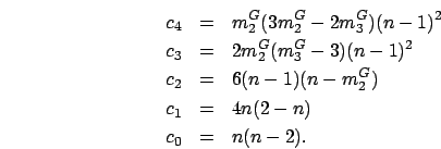
$f$ is a solution for the fourth order equation 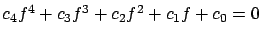$c_4f^4+c_3f^3+c_2f^2+c_1f+c_0=0$, where

$$\begin{eqnarray*} c_4 & = & m_2^G (3m_2^G-2m_3^G)(n-1)^2 \\ c_3 & = & 2 m_2^G... ... 6(n-1)(n-m_2^G) \\ c_1 & = & 4n(2-n) \\ c_0 & = & n(n-2). \end{eqnarray*}$$

.
.
.
.
.
.
.
.
.
.
.
.
.
.
.
.
.
.
.
.
.
.
.
.
.
.
.
.
.
.