Analysis of Algorithms

We want to be able to analyze algorithms, not just the methods that implement them. That means we should be able to say something interesting about the performance of an algorithm independent from having a version of it (written in some programming language) that a machine can execute. Once we examine machine-executable versions, there is a lot of technology details to deal with: what language we write the code in, which compiler we use for that language, what speed processor we run it on, how fast memory is (and even how much caching is involved). While this information is important to predict running times, it is not fundamental to analyzing the algorithms themselves. So, we will analyze algoritms independent of technology, making this subject more scientific.

Instead, we will analyze an algorithm by predicting how many steps it takes, and then go through a series of simplifications leading to characterizing an algorithm by its complexity class. Although it initially may seem that we have thrown out useful information, we will learn how to predict running times of methods on actual machines, using an algorithm's complexity class, and timing it on the machine that it will be run on.

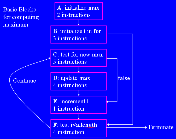
  int max = Integer.MIN_VALUE;
  for (int i=0; i<a.length; i++)
    if (a[i] > max)
      max = a[i];

We can easily examine the machine language instructions that Java produces for this code by using the debugger. If we specify Mixed on the bottom control of its window, Java shows us the Java code interspersed with the machine language instructions.

Below, I have duplicated this information, but reformatted it to be more understandable. I have put comments at the end of every line and put blank lines between what compiler folks call basic blocks.

          int max = Integer.MIN_VALUE;                          : A
051E6B3D: 1209           ldc       (#9) 
051E6B3F: 3D             istore_2

          for (int i=0; i<a.length; i++)
051E6B40: 04      iconst_0               //get 0                : B
051E6B41: 3E      istore_3               //  store it in i
051E6B42: A70011  goto      0x051E6B53   //go to test near bottom

          if (a[i] > max)
051E6B45: 2B      aload_1                //get a's base address : C
051E6B46: 1D      iload_3                //  get i
051E6B47: 2E      iaload                 //  get a[i]
051E6B48: 1C      iload_2                //get max
051E6B49: A40007  if_icmple  0x051E6B50  //go to test near bottom if <=

          max = a[i];		
051E6B4C: 2B      aload_1                //get a's base address : D
051E6B4D: 1D      iload_3                //  get i
051E6B4E: 2E      iaload                 //  get a[i]
051E6B4F: 3D      istore_2               //store it in max

051E6B50: 840301  iinc      3 1          //increment i          : E

051E6B53: 1D      iload_3                //get i                : F
051E6B54: 2B      aload_1                //get a's
051E6B55: BE      arraylength            //  length
051E6B56: A1FFEF  if_icmplt  0x051E6B45  //go to if above if <

Each basic block can be entered only at the top and exited only at the bottom. once a basic block is entered, all its instructions are executed. There may be multiple ways to enter and exit blocks. This code is a bit tortuous to read and hand simulate, but you can trace through it. An easier way to visualize the code in these basics blocks is as a graph, which I will annotate with all the information needed to understand computing instruction counts from it.

If the array contains 0 values, 9 instructions are executed: blocks A, B, F. If the array contains 1 value, 23 instructions are executed: blocks A, B, F, C, D, E, F. If the array contains 2 values, either 33 instructions are executed (the first value is bigger than the second: blocks A, B, F, C, D, E, F, C, E, F) or 37 instructions are executed (the second value is bigger than the first - the worst case: A, B, F, C, D, E, F, C, D, E, F). Assuming the worst case from now on, if the array contains 3 values, 51 instructions are executed. ...

Thus, for this example -the code to compute the maximum value in an array- we can write the formula. Iaw(N) = 14N + 9. At most there are 14 instructions executed during each loop iteration (blocks C, D, E, F); the housekeeping to initialize max and initialize i and check the first loop iteration requires 9 instructions (blocks A, B, F). In fact, computing Iab (the number of steps in the best case, where the if test is true only on the first iteration, is

  Iab(N) = 14N + 9 - 4(N-1) = 10N + 13

Here N is a.length (the number of values stored in the array), and the worst-case run will be on an array of strictly increasing values: the if test executed during each iteration of the loop is repeatedly true, so the machine instructions to copy that value into max (block D) are always executed. Determining the average case is a problem in discrete math: given a random distribution (there are many; say the numbers are distributed uniformly) of values, how many times (on average) do we expect to execute block B, meaning the next value to be bigger than all the prior ones; this is not a simple problem but we can write programs to help understand it.

Let's return our focus to Iaw(N) = 14N + 9. Although this formula is simple, we want to make it even simpler if we can. Note that as N gets large (and most algorithmic analysis is asymptotic: it is concerned with what happens as the problem size N gets very large), the lower order term (9) can be dropped from this function to simplify it (less precision), without losing much accuracy.

For example, if N is 100, Iaw(N) = 1,409: if we drop the 9 term, the simplified answer is just 1,400 which is 99.3% of the correct answer; if we increase N to 1,000, Iaw(N) = 14,009: if we drop the 9 term, the simplfied answer is just 14,000 which is 99.94% of the correct answer; if we increase N to 10,000, Iaw(N) = 140,009: if we drop the 9 term, the simplfied answer is just 140,000 which is 99.994% of the correct answer.

Thus as N gets large (and 10,000 is not even a very large problem for computers) the lower term is not significant so we will drop it to simplify the formula to Iaw(N) = 14N.

Mathematically, if Td(N) is the dominant term (here 14N, we can drop any term T(N) if T(N)/Td(N) -> 0 as N -> infinity: note that 9/14N -> 0 as N -> inifinity, so that term can be dropped.

  for (int base=0; base<N; base++)
    for (int check=base+1; check<N; check++)
      if (a[base]>a[check]) {
        int temp = a[base];
        a[base]  = a[check];
        a[check] = temp;
      }

If the array contains 0 values, 7 instructions are executed: blocks A, H. If the array contains 1 value, 21 instructions are executed: blocks A, H, B, F, G, H. If the array contains 2 values, 63 instructions are executed: blocks A, H, B, F, C, D, E, F, G, H, B, F, I, H. If the array contains 3 values, 133 instructions are executed The resulting instruction-counting function is

  Iaw(N) = 28N(N-1)/2 + 14N +7 = 14N2 + 7

Recall our terms T(N) can be dropped if the limit T(N)/Td(N) -> 0 as N -> infinity: note that 7/14N² -> 0 as N -> inifinity, so that term can be dropped.

Now, let's take a look at the constant in front of the dominant term; it's value doesn't really matter for three important reasons. And, by getting rid of it we can simplify the formula again.

1. First, when computing the run time we are just going to multiply this constant by another constant relating to the machine, so we can discard this constant if we just use a different constant for the machine. Let Taw(N) denote the time taken by algorithm by algorithm a when run on the worst-case problem of size N. If our machine executes 2 billion instructions/second, then the formula in the second case is Taw(N) = 14N²/2x10⁹, or Taw(N) = .000000014N².

2. Second, a major question that we want answered is how much extra work does an algorithm do if the size of a problem is doubled. Note that for the second simplified version of Iaw (the one with only the dominant term multiplied by a constant), Iaw(2N)/Iaw(N) = 14(2N)² / 14N² = 4 (meaning doubling the problem size quadruples the number of instructions that this algorithm executes), so the constant is actually irrelevant to the computation of this ratio.

3. Third, a major question that we want answered is how the speed of two algorithms compare: specifically, we want to know whether Iaw(N)/Ibw(N) -> 0 as N -> infinity, which would mean that algorithm a gets faster and faster compared to algorithm b. Again, the constant is irrelevant to this calculation.

Big O notation doesn't tell us everything that we need to know about the running time of an algorithm. For example, if two algorithms are O(N²), we don't know which will eventually become faster). And, if one algorithm is O(N) and another is O(N²), we don't know which will be faster for samll N. But, it does economically tell us quite a bit about the performance of an algorithms (see the three important questions above). We can compute the complexity class of an algorithm by the process shown above, or by doing something much simpler: determining how often its most frequently executed statement is executed as a function of N.

Returning to our first example,

  int max = Integer.MIN_VALUE;
  for (int i=0; i<a.length; i++)
    if (a[i] > max)
      max = a[i];

the if statement is executed N times, where N is the length of the array: a.length.

Returning to our second example,

  for (int base=0; base<N; base++)
    for (int check=base+1; check<N; check++)
      if (a[base]>a[check]) {
        int temp = a[base];
        a[base]  = a[check];
        a[check] = temp;
      }

Finally, note that comparing algorithms by their complexity classes is useful only for large N. We cannot state authoritatively whether an O(N) algorithm or an O(N²) algorithm is faster for small N; but we can state that once we pass some threshold for N (call it N₀), the O(N) algorithm will always be faster than the O(N²) algorithm. This ignorance is illustrated by the picture below.

Technically, an algorithm a is O(f(n)) if and only if there exist a number M and N₀ such that Iaw(n) <= Mf(n) for all n>N₀ This means for example that any O(N) algorithm is also O(N²) too (or O(f(n)) for any f(n) that grows faster than linearly). Technically Ω is the symbol to use when you know a tight bound on both sides: if there exists M₁, M₂, and N₀ such that M₁f(n) <= Iaw(n) <= Mf(n) for all n>N₀, we say that algorithm a is Ω(f(n)). We will use just Big O notation, often pretending it is Ω. See Big O Notation in the online Wikipedia for more details.

For example, if a method implementing a certain sorting algorithm is in the complexity class O(N²), and it takes about 1 second to sort 10,000 values, it will take about 4 seconds to sort 20,000 values. That is, for complexity class O(N²), doubling the size of the problem quadruples the amount of time taken executing a method. The algebra to prove this fact is simple. Assuming Taw(N) = c*N² (where c is some technology constant related to the compiler used, the speed of the computer and its memory, etc.) the ratio of the time taken to solve a problem of size 2N to the time take to solve a problem of size N is.

  Taw(2N)/Taw(N) = c*(2N)2 / c*(N)2 = 4cN2 / cN2 = 4

Likewise, using this method to sort 1,000,000 values (100 times more data) would take about 2.8 hours (that is 10,000 times longer, which is 100²).

Here is a short characterization of some common complexity classes (there are many others: any expression that is a formula using N). We will discuss some of these algorithms in more detail later in this handout, and use these complexity class to characterize many methods throughout the semester.

Complexity Class	Class Name	Example	T(2N)
O(1)	Constant	Insertion at the rear of an array Insertion at front of linked list Parameter passing	T(N)
O(log2N)	Logarithmic	Binary Search	T(N)+constant
O(N)	Linear	Linear Search (arrays or linked lists)	2T(N)
O(N log2N)	Log-Linear or Linearithmic	Fast Sorting	2T(N)+constant
O(N2)	Quadratic	Slow/Simple Sorting	4T(N)
O(N3)	Cubic	NxN Matrix Multiplication	8T(N)
O(NC)	Polynomial or Geometric		2cT(N)
...	...	...	...
O(CN)	Exponential	Proving Boolean Equivalences of N variables	CNT(N)

We can compute log₂N = (ln N)/(ln 2) = 1.4427 ln N. Since log base 2 and log base e are linearly related, it really makes no difference which we use when using Big O notation, because only the constants (which we ignore) are different. You should also memorize that log₂1000 is about 10 (actually log₂1024 is exactly 10), and that log₂N^a = alog₂N. From this fact we can easily compute log₂1,000,000 as log₂1,000² which is 2log₂1000 which is about 20. Do this for log₂1,000,000,000 (one billion).

Again, we should understand that these simple formulas work only when N gets large. This is the core of asymptotic algorithmic analysis Note that complexity classes before (and including) log-linear are considered "fast": their running time does not increase much faster than the size of the problem increases. The later complexity classes O(N²), O(N³), etc. are slow but "tractable". The final complexity class O(2^N) grows so fast that it is called "intractable": only small problems in this complexity class can ever be solved.

For example, assume that Ia₁w(N) = 10 (constant), and Ia₂w(N) = 10log₂N (logrithmic), and Ia₃w(N) = 10N (linear), etc. Assume further that we are running code on a machine executing 1 billion (10⁹) operations per second. Then the following table gives us an intuitive idea of how running times for algorithms in different complexity classes changes with problem size.

Complexity Class	N = 10	N = 100	N = 1,000	...	N = 1,000,000
O(1)	1x10-7 seconds	1x10-7 seconds	1x10-7 seconds	...	1x10-7 seconds
O(log2N)	3.3x10-7 seconds	6.6x10-7 seconds	10x10-7 seconds	...	20x10-7 seconds
O(N)	1x10-7 seconds	1x10-6 seconds	1x10-5 seconds	...	1x10-3 seconds
O(Nlog2N)	3.3x10-7 seconds	6.6x10-6 seconds	10x10-5 seconds	...	20x10-3 seconds
O(N2)	1x10-6 seconds	1x10-4 seconds	1x10-2 seconds	...	2.7 hours
O(N3)	1x10-5 seconds	1x10-2 seconds	10 seconds	...	3x103 years
O(2N)	1x10-5 seconds	4x1021 centuries	fuggidaboutit	...	fuggidaboutit

For a first example, we will measure, and then predict, the running time of a simple, quadratic sorting method. We will use a driver program (discussed below, in the Sorting section) to repeatedly sort an array containing 1,000 random values, and then predict how long it will take this method to sort an array containing of 10,000 random values (and actually compare this prediction to the measured running time for this problem size).

1. Because this sorting method is in the O(N²) complexity class, we simply assume that we can write T(N) = cN² where we do not know the value of c yet.
2. We run the sorting method five times on an array containing 1,000 random values and measure the average running time: it is .022 seconds.

  T(1000) = c 10002
.022    = c 106
c       = .022/106
c       = 2.2 x 10-8

For a second example, we wil measure, and then predict, the running time of a more complicated log-linear sorting method (this algorithm is in the lowest complexity class for all those that accomplish sorting). We will use a driver program to repeatedly sort an array containing 100,000 random values, and then predict how long it will take this method to sort an array containing of 1,000,000 random values (and actually compare this prediction to the measured running time for this problem size, which is small enough to measure).

1. Because this sorting method is in the O(N log₂N) complexity class, we simply assume that we can write T(N) = c(N Log₂N) where we do not know the value of c yet.
2. We run the sorting method five times on an array containing 100,000 random values and measure the average running time: it is .15 seconds (notice that this method sorts 10 times as many values over 10 times faster than the simple quadratic sorting method on the same amount of data).

T(100,000) = c (1,000,000 log 2 1,000,000)
.15        = c 1,660,964
c          = .15/1,660,964
c          = 9.0 x 10-9

Here is a final word on the accuracy of our predictions. If we sort the exact same array a few times (the sort testing driver easily does this) we will see variations of 10%-20%; likewise we get a slightly greater spread if we sort different arrays (but all of the same size). Our model predicts that these would all take the same amount of time. So all kinds of things (operating system, what programs it is running, what network connections are open, etc.) influence the actually amount of time taken to sort an array. In this light, the accuracy of our "naive" predictions is actually quite good.

First, be aware that the standard timer in Java is accurate to only .001 second (1 millisecond). Call this one tick So, to get any kind of accuracy, you should run the method on large enough data to take tens to hundreds of ticks (milliseconds).

So, run the method on some data of size N, enough for the required number of ticks, then of size 2N, then of size 4N, then of size 8N. For algorithms in simple complexity classes, you should be able to recognize a pattern (which will be approximate by not exact). If the sequence of values is 1.0 seconds, 2.03 seconds, 3.98 seconds, and 8.2 seconds: the method seems O(N). Here each doubling approximately doubled the time the method ran. If the sequence of values is 1.0 seconds, 3.8 second, 17.3 seconds, and 70.3 seconds: the method seems O(N²). Here each doubling approximately quadrupled the time the method ran.

Of course, things get a bit subtle for a complexity class like O(Nlog₂N), but you'll see it always a bit worse than linear, but nowhere near quadratic. Of course O(Nlog²₂N) would behave simlarly, so you must apply this process with a bit of skepticism that you are computing perfect answers.

  public static int linearSearch (int[] a, int value)
  {
    for (int i; i<a.length; i++)
      if (a[i] == value)
        return i;
    return -1;
  }

Let's explore this algorithm first in a more physical context. Suppose that we have 1,000,000 names in alphabetical (sorted) order in a phone book, one name and its phone number per page (only on the front of a page, not the back). Here is an algorithm to find a person's name (and their related phone number) in such a phone book

1. Find the middle page in the (remaining) book
2. If it contains the name that we are looking for, we are done
3. Otherwise, we rip out that page and tear the remaining phone book in half
   1. If the name we are looking for comes before the page we that ripped out, we throw away the second half of the phone book
   2. If the name we are looking for comes after the page that we ripped out, we throw away the first half of the phone book
4. Repeat this process until we find the name or there are no pages left in the phone book

If the original phone book had 1,000,000 pages, after the first iteration (assuming the name we are looking for isn't right in the middle) the remaining book would have about 500,000 pages (actually it would have 499,999). In this algorithm, the first comparison eliminates about 500,000 pages! After the second comparison, we are down to a phone book containing about 250,000 pages. Here one more comparison eliminates about 250,000 pages; not as good as the first comparison, but still much better than linear searching, where each comparison eliminates just one page! If we keep going, we’ll either find the name or after about 20 comparisons the phone book will be reduced to have no pages. Critical to this method is the fact that the phone book is alphabetized (ordered); it is also critical to be able to find the middle of the phone book quickly (which is why this method doesn't work on linked lists).

To determine the complexity class of this algorithm (operating on a sorted array), notice that each comparison cuts the remaining array size in half (actually, because the midpoint is also eliminated with the comparison, the size is cut by a bit more than a half). For an N page book, the maximum number of iterations log₂ N (the number of times we can divide N by 2 before it is reduced to 1; or, the number of times that we can double 1 before reaching N). Notice in this algorithm if the array size doubles, the number of iterations increases by just 1: the first comparison would cut the doubled array size back to the original array size.

Again, here are some important facts about logarithms that you should memorize.

1. 2¹⁰ = 1,024 so log₂ 1,000 is about 10
2. log₂ X² = 2 log₂ X; so log₂ 1,000,000 = log₂ 1000² = 2 log₂ 1000 is about 20
3. On a calculator, compute log₂ N = ln N / ln 2 (where ln is logarithm base e, provided on most calculators -and by the Math.log method).

Here a method for implementing the binary search algorithm on arrays.

  public static int binarySearch (int[] a, int value)
  {
    int low  = 0;
    int high = a.length-1
    for(;;) {
      if (low > high)           //low/high bounds inverted, so
        return -1;              //  the value is not in the array

      int mid = (low+high)/2;   //Find middle of the array

      if (a[mid] == value)      //Found value looking for, so
        return mid;             //  return its index; otherwise
      else if (value < a[mid])  //determine which half of the
        high = mid-1;           //  array potential stores the
      else                      //  value and continue seraching
        low  = mid+1;           //  only that part of the array
  }

Finally, note that we cannot perform binary searching efficiently on linked lists, because we cannot quickly find the middle of a linked list. In fact, another self-referential data structure, trees, can be used to perform efficient searches.

Here is a brief description of three O(N²) sorting algorithms.

1. In bubble sort, a next position to fill is compared with all later positions, swapping out-of-order values.
2. In selection sort, the smallest value in the remaining positions is computed and swapped with the value in the next position.
3. In insertion sort, the next value is moved backward (swapped with the value in the previous position in the region of sorted values) until it reaches its correct position.

Here is a brief description of three O(N log₂ N) sorting algorithms.

1. In merge sort, pairs of small, adjacent ordered arrays (the smallest are 1 member arrays) are merged repeated into larger ordered arrays until the result is just one ordered array containing all the values.
2. In heap sort, values are added to and then removed from a special kind of tree data structure called a heap (which we will study later: its add and remove operations are both O(log₂ N), so adding and then removing N values is NxO(log₂ N) + NxO(log₂ N) = O(N log₂ N) total.
3. In quick sort, a pivot value is chosen and then the array is partitioned into three regions: on the left are those values less than the pivot, in the middle are those equal to the pivot, and on the right are those values greater than the pivot; then this process is repeated in the left and right regions (if they contain more than one value).

All these sorting algorithms are defined as static methods in the Sort class. All method have exactly the same prototype (so they can be easily interchanged)

  public static void bubble (Object[] a, int size, Comparator c)

1. An array of Object references to be sorted.
2. An int specifying how many references are stored in the array; this can be a.length if the array is filled.
3. An object from a class implementing Comparator, which decides which objects belong before which others in the sorted array.

Finally, it has been proven that when using comparisons to sort values, all algorithms require at least O(N log₂ N) comparisons. Thus, there are no general sorting algorithms in any complexity class smaller than log-linear (although better algorithms -ones with smaller constants- may exist).

So, in the case of simple array implementations of a stack or queue, both "add" methods (push and enqueue) are O(1) (assuming no new memory must be allocated); but the pop remove method is O(1) while the dequeue) remove method is O(N). Because NxO(1) is O(N), and O(N)+O(N) is O(N), adding and then removing N values from the stack collection classes is O(N). Because NxO(N) is O(N²), and O(N)+O(N²) is O(N²), adding and then removing N values from the queue collection classes is O(N²).

As another example, look at the array implementation of a simple priority queue, keeping the array sorted. There, the enqueue operation is O(N) because this method scans the array trying to find the correct position (based on its priority; highest priority is at the rear) for the added value. In the worst case, it has a priority lower than any other value, so the entire array must be moved backward to put that value at the front. The dequeue operation is just O(1), because it just removes the value at the rear of the array, requiring no other data movement. Because NxO(N) is O(N²), and NxO(1) is O(N), and O(N²)+O(N) is O(N²), adding and then removing N values from this implementation of a priority queue also has a complexity class O(N²).

If we instead enqueued the value on the rear and dequeued by searching through the array for the highest priority value, we would still have one O(N) term and one O(N²) term, leading to O(N²) as the overall complexity class. But, later we will learn how implement priority queues with heaps. Both enqueue and dequeue are O(log₂N): worse than O(1) but better than O(N). Thus, adding and then removing N values from this implementation of a priority queue is NxO(log₂N) + NxO(log₂N) which is O(Nlog₂N) + O(Nlog₂N) which is O(Nlog₂N). So, "balancing" the add and remove operations yields a lower complexity class when both operations occur N times.

Finally, when we use an array to store a collection, each time that we double the array we must copy its N values. By doubling the size, we do this only log₂ N times when adding N values, for a total of Nlog₂N copies; therefore, we can think of each addition as requiring log₂N copies (this is called the "amortized cost" of this operation: it really doesn't occur on every add, but when averaged over all the adds it is correct). So, in the case of an array implementation of a stack or queue, both "add" methods are actually O(log₂ N). Because NxO(log₂ N) is O(N log₂ N), NxO(1) is O(N), and NxO(N) is O(N²), The stack class is actually O(N log₂ N) for N pushes and pops, while the stack class is actually O(N²) for N enqueues and dequeues. By this calculation, the array implementations have a slightly higher complexity class than those using linked lists. But, because linked lists allocated a new object for every value put in the linked list, the running time of collections using linked lists can actually be higher. We will address this problem again when we cover linked lists.

Programs should run as fast as necessary; making a program run faster often requires making it more complicated, more difficult to generalize, etc. For example, many scientific programs run in just a few seconds. Is there a pragmatic reason to work on them to run faster? No, because it typically takes a few days to collect the data for the program. As a component in the entire task, the program part is already fast enough. Likewise, programs that require lots of user interaction don't need to be made more efficient: if the computer spends less than a tenth of a second between the user entering his/her data and the program prompting for more, it is fast enough. Finally, in the pinball animation program, if the model can update and show itself in less than a tenth of a second, there is no reason to make it run faster; if it cannot, then the animation will be slowed down, and there is a reason to improve its performance.

The most famous of all rules of thumb for efficiency is the rule of 90/10. It states that 90% of the time a program takes to run is a result of executing just 10% of its code. That is, most time in a program's execution is spent in a small amount of its code. Modifying this code is the only way to achieve any significant speedup.

For example, suppose a 10,000 line program runs in 1 minute. By the rule of 90/10, executing 1,000 lines in this program accounts for 54 seconds, while executing the remaining 9,000 lines account for only 6 seconds. So, if we could locate and study those 1,000 lines (a small part of the program) and get them to execute in half the time, the total program would run in 27+6 = 33 seconds, which reduces the execution time for the entire program by almost 50%. If instead we could study the other 9,000 lines and get them to execute instantaneously (admittedly, a very difficult feat!), the total program would run in 54+0 = 54 seconds, which reduced the execution time for the entire program by ony 10%. Note that if you randomly change code to improve its efficiency, 90% of the time you will not be making any changes resulting in a significant improvement.

Thus, a corollary of the 90/10 rule is that for 90% of the code in a program, if we make it clearer but less efficient, it will not affect the total execution time of the program by much. In the above program, if we rewrote the 9,000 lines to make them as clear and simple as possible (with no regard for their efficiency) and increased their running time by 50% (from 6 to 9 seconds), the total program would run in 54+9 = 63 seconds, which is only a 5% increase in total execution time.

Java has a very simple (but not so useful) built-in profiler. To use it, select Edit from the Metrowerks CodeWarrior toolbar, then select Java Application Release Setting. In the Target Settings Panel, click on Java Target and in the VM Arguments text field, enter -Xrunhprof:cpu=times as is illustrated below.

Typically one can speed up a program by a factor of 3-10 very quickly. Further gains are slow, unless algorithms from lower complexity classes can be found.

If you get stumped on any problem, go back and read the relevant part of the lecture. If you still have questions, please get help from the Instructor, a CA, or any other student.

1. When we say an algorithm is O(1) what do we mean?

2. Where does the complexity class O( N sqrt(N) ) fit in the hierarchy shown in this lecture?

3. Suppose that the actual time taken to execute an O(N²) sorting algorithm on a very fast machine is 2.2x10^-8N² seconds; now suppose that the actual time taken to execute an O(N log₂ N) sorting algorithm on a very slow machine is 7.2x10^-4(N log₂ N) seconds (here the slow machine is about 10,000 slower than the fast one). For what size arrays will the slower machine running the faster algorithm sort arrays faster than the faster machine running the slower algorithm?

4. Suppose that my Sort class has two methods

     public static void sortByMethod1(Object[] a, Comparator c);
     public static void sortByMethod2(Object[] a, Comparator c);

   After testing these methods exhaustively, we find that the first method works faster than the second for all arrays whose length is less than 13, and the second works faster for all bigger arrays. Write a method name superSort that has the same prototype and always runs as fast as the fastest of these two methods.

5. Rexamine the code for the first example, computing the maximum value stored in an array. There is one value (hint: final) that is recomputed, but it never changes; we could instead write code that is a bit more verbose, but executes fewer machine language instructions. Identify the redundancy, write the Java code to fix it, and determine Iaw(N) for the new program. You might check your result using Mixed mode in the debugger. If the body of the loop were longer, would this improvement have a bigger or lesser effect overall?

6. Write a program that fills an array of length N with random values. Then run the maximum code, incrementing a counter whenever a new maximum is found. Run this program for large values of N and try to infer a formula for that approximates how many times this happens. Run the program over and over again, with the same large N, then with double that size, quadruple that size, etc. to test your formula.