In this section we apply the scheduling algorithm from
Section 2 to route N packets in ![]() steps on an N-node butterfly using constant size queues. We
essentially duplicate the result of Ranade [29], but the
proof is simpler.
steps on an N-node butterfly using constant size queues. We
essentially duplicate the result of Ranade [29], but the
proof is simpler.
In a butterfly network, each node has a distinct label ![]() , where l is its level and r is its row. In an
n-input butterfly, l is an integer between 0 and
, where l is its level and r is its row. In an
n-input butterfly, l is an integer between 0 and ![]() , and
r is a
, and
r is a ![]() -bit binary number. The nodes on level 0 and
-bit binary number. The nodes on level 0 and ![]() are called the inputs and outputs, respectively. Thus, an
n-input butterfly has
are called the inputs and outputs, respectively. Thus, an
n-input butterfly has ![]() nodes. For
nodes. For ![]() , a
node labeled
, a
node labeled ![]() is connected to nodes
is connected to nodes ![]() and
and ![]() , where
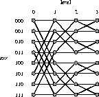
, where ![]() denotes r with the lth bit complemented. An 8-input butterfly
network is illustrated in Figure 3. Sometimes the
input and output nodes in each row are identified as the same node.
In this case the number of nodes is
denotes r with the lth bit complemented. An 8-input butterfly
network is illustrated in Figure 3. Sometimes the
input and output nodes in each row are identified as the same node.
In this case the number of nodes is ![]() . The butterfly has
several natural recursive decompositions. For example, removing the
nodes on level 0 (or
. The butterfly has
several natural recursive decompositions. For example, removing the
nodes on level 0 (or ![]() and their incident edges leaves two
and their incident edges leaves two
![]() -input subbutterflies.
-input subbutterflies.

Figure 3: An 8-input butterfly
network. Each node has a level number between 0 and 3, and a
3-bit row number. A node on level l in row r is connected to
the nodes on level l+1 in rows r and ![]() , where where
, where where
![]() denotes r with the lth bit complemented.
denotes r with the lth bit complemented.
![]()
Proof:
Routing is performed on a logical network consisting of ![]() levels. The first
levels. The first ![]() levels of the logical network are linear
arrays. The packets originate in these arrays, one to a node. Levels
levels of the logical network are linear
arrays. The packets originate in these arrays, one to a node. Levels
![]() through
through ![]() form a butterfly network. Levels
form a butterfly network. Levels ![]() through
through ![]() consist of a butterfly with its levels reversed.
The last
consist of a butterfly with its levels reversed.
The last ![]() levels are again linear arrays. Each packet has its
destination in one of the arrays spanning levels
levels are again linear arrays. Each packet has its
destination in one of the arrays spanning levels ![]() to
to ![]() . Packets with the same destination are combined. The butterfly
simulates each step of this logical network in a constant number of
steps. Paths for the packets are selected using Valiant's paradigm;
each packet travels to a random intermediate destination on level
. Packets with the same destination are combined. The butterfly
simulates each step of this logical network in a constant number of
steps. Paths for the packets are selected using Valiant's paradigm;
each packet travels to a random intermediate destination on level
![]() before moving on to its final destination. This strategy
ensures that with high probability, say at least
before moving on to its final destination. This strategy
ensures that with high probability, say at least ![]() , where
, where
![]() is a constant, the congestion is
is a constant, the congestion is ![]() . Since the paths
are chosen independently of the ranks for the packets, the scheduling
algorithm can treat the paths as if they were fixed. Assuming that
the paths have congestion
. Since the paths
are chosen independently of the ranks for the packets, the scheduling
algorithm can treat the paths as if they were fixed. Assuming that
the paths have congestion ![]() , by Theorem 2.9
the scheduling algorithm delivers all of the packets in
, by Theorem 2.9
the scheduling algorithm delivers all of the packets in ![]() steps, with high probability, say at least
steps, with high probability, say at least ![]() . Thus, the
probability that either the congestion is too large or that the
scheduling algorithm takes too long to deliver the packets is at most
. Thus, the
probability that either the congestion is too large or that the
scheduling algorithm takes too long to deliver the packets is at most
![]() .
.

Proof:
If each input sends a single packet, the congestion will be
![]() , with high probability. Given paths with
congestion
, with high probability. Given paths with
congestion ![]() , by Theorem 2.9
the delay is
, by Theorem 2.9
the delay is ![]() , with high probability.
, with high probability.