4.1 Comparison of the q_g and q_c Heuristics

Our experience in different medical applications indicates that intuitions like ``how expensive is every FP prediction in terms of additional TP predictions made by a rule'' are useful for understanding the problem of directing the search in the TP/FP space. Suppose that the definition of cost parameter c is based on the following argument: ``For every additional FP, the rule should cover more than c additional TP examples in order to be better.'' Based on such reasoning, it is possible to define a quality measure q_c, using the following TP/FP tradeoff:

$$q_{c} = TP - c \cdot FP.$$

Quality measure q_c is easy to use because of the intuitive interpretation of parameter c. It has also a nice property when used for subgroup discovery: by changing the c value we can move in the TP/FP space and select the optimal point based on parameter c.

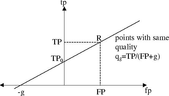
In Algorithm SD, the quality measure q_g, using a different TP/FP tradeoff is used: q_g = TP/(FP+g), where g is the generalization parameter.

If a subgroup discovery algorithm employs exhaustive search (or if all points in the TP/FP space are known in advance) then the two measures q_g and q_c are equivalent in the sense that every optimal solution lying on the convex hull can be detected by using any of the two heuristics; only the values that must be selected for parameters g and c are different. In this case, q_c might be even better because its interpretation is more intuitive.

However, since Algorithm SD is a heuristic beam search algorithm, the situation is different. Subgroup discovery is an iterative process, performing one or more iterations (typically 2-5) until good rules are constructed by forming conjunctions of features in the rule body. In this process, a rule quality measure is used for rule selection (for which the two measures q_g and q_c are equivalent) as well as for the selection of features and their conjunctions that have high potential for the construction of high quality rules in subsequent iterations; for this use, rule quality measure q_g is better than q_c. Let us explain why.

Suppose that we have a point (a rule) R in the TP/FP space, where TP and FP are its true and false positives, respectively. For a selected g value, q_g can be determined for this rule R. It can be shown that all points that have the same quality q_g as rule R lie on a line defined by the following function:

$$tp = \frac{TP \cdot fp}{FP + g} + \frac{TP \cdot g}{FP + g} = \frac{TP \cdot (fp + g)}{FP + g}.$$

In this function, tp represents the number of true positives of a rule with quality q_g which covers exactly fp negative examples. By selecting a different fp value, the corresponding tp value can be determined by this function. The line, determined by this function, crosses the tp axis at point $TP_{0} = TP \cdot g/(FP+g)$ and the fp axis at point -g. This is shown in Figure 11. The slope of this line is equal to the quality of rule R, which equals TP/(FP+g).

Figure 11: Properties of rules with the same quality q_g.

Figure 12: Rules with highest quality included into the beam for q_g = TP/(FP+g).

In the TP/FP space, points with higher quality than q_g are above this line, in the direction of the upper left corner. Notice that in the TP/FP space the top-left is the preferred part of the space: points in that part represent rules with the best TP/FP tradeoff. This reasoning indicates that points that will be included in the beam must all lie above the line of equal weights q_beam which is defined by the last rule in the beam. 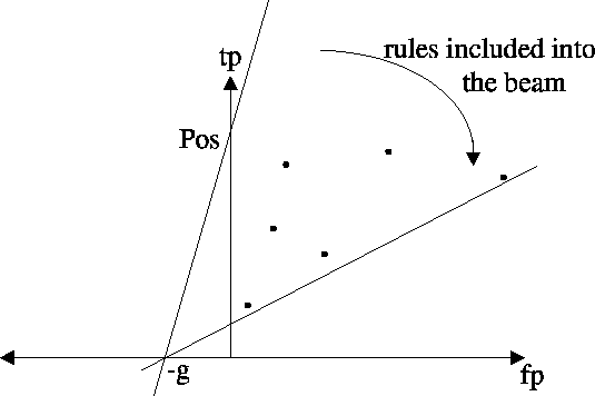If represented graphically, first $beam\_width$ number of rules, found in the TP/FP space when rotating the line from point (0,Pos) in the clockwise direction, will be included in the beam. The center of rotation is point (-g,0). This is illustrated in Figure 12.

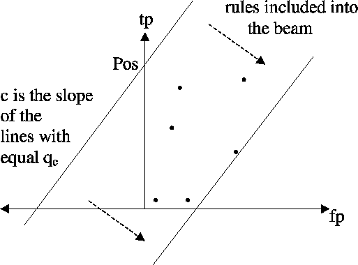
On the other hand, for the q_c quality measure defined by $q_{c} = TP - c \cdot FP$ the situation is similar but not identical. Points with the same quality lie on a line $tp=c \cdot (fp-FP)+TP$, but its slope is constant and equal to c. Points with higher quality lie above the line in the direction of the left upper corner. The points that will be included into the beam are the first $beam\_width$ points in the TP/FP space found by a parallel movement of the line with slope c, starting from point (0,Pos) in the direction towards the lower right corner. This is illustrated in Figure 13.

Figure 13: Rules with highest quality included in the beam for $q_{c} = TP - c \cdot FP$.

Figure 14: Placement of interesting features in the TP/FP space after the first iteration.

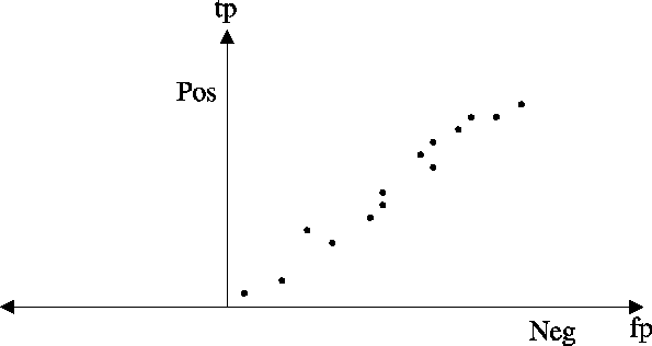
Let us now assume that we are looking for an optimal rule which is very specific. In this case, parameter c will have a high value while parameter g will have a very small value. The intention is to find the same optimal rule in the TP/FP space. At the first stage of rule construction only single features are considered and most probably their quality as the final solution is rather poor. See Figure 14 for a typical placement of potentially interesting features in the TP/FP space.

The primary function of these features is to be good building blocks so that by conjunctively adding other features, high quality rules can be constructed. By adding conjunctions, solutions generally move in the direction of the left lower corner. The reason is that conjunctions can reduce the number of FP predictions. However, they reduce the number of TP's as well. Consequently, by conjunctively adding features to rules that are close to the left lower corner, the algorithm will not be able to find their specializations nearer to the left upper corner. Only the rules that have high TP value, and are in the upper part of the TP/FP space, have a chance to take part in the construction of interesting new rules.

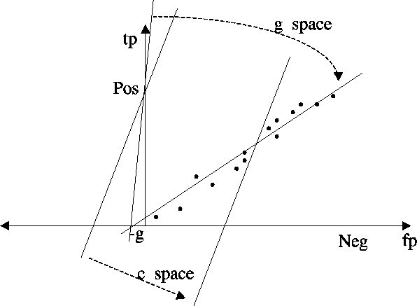
Figure 15 illustrates the main difference between quality measures q_g and q_c: the former tends to select more general features from the right upper part of the TP/FP space (points in the so-called `g space'), while the later `prefers' specific features from the left lower corner (points in the so-called `c space'). In cases when c is very large and g is very small, the effect can be so important that it may prevent the algorithm from finding the optimal solution even with a large beam width. Notice, however, that Algorithm SD is heuristic in its nature and no statements are true for all cases. This means that in some, but very rare cases, a quality measure based on parameter c may result in a better final solution.

Figure 15: The quality q_c employing the c parameter tends to select patterns (points) with small TP values, while quality q_g employing the g parameter will include also many patterns with large TP values (from the right part of the TP/FP space) that have a chance to be used in building conjunctions of high quality rules.