 |
A bi-partite graph is a network consisting of two layers of nodes, where the top layer is hidden and the bottom layer visible. The only connections in the network are from the top layer (parent nodes) to the bottom layer (child nodes). Such a architecture appears very simple, but already with several tens of nodes it is often intractable to compute the marginals exactly when evidence is presented. A bi-partite graph can be undirected or directed (pointing downwards). A recent example of the first is the PoE (product of experts) from hinton99a with discrete nodes. The `Quick Medical Reference' (QMR) network from shwe91a is a good example for a directed bi-partite graph. Recently there were some approaches to use approximation techniques for this network jaakkola99variational,murphy99a. Therefore we have chosen to use the bi-partite network as an architecture to test the bound propagation algorithm on.
We created bi-partite networks of an equal number of (binary valued) nodes in both layers. Each child node has exactly three parents and each parent points to exactly three children. The connections were made randomly. The conditional probability tables (CPT's) holding the probability of the child given its parents was initialized with uniform random number between zero and one. The prior probability tables for the parents were initialized similarly.
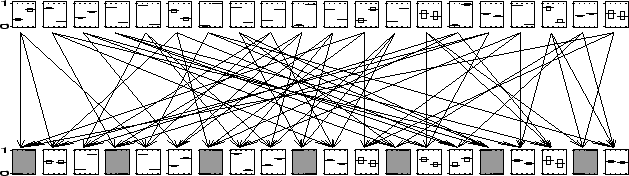
In Figure ![[*]](crossref.png) we show a bi-partite network with twenty nodes in
each layer, which is still small enough to compute the exact marginals.
The arrows show the parent-child relations. To every third child evidence
was presented (the shaded nodes). We ran the bound propagation algorithm
with
we show a bi-partite network with twenty nodes in
each layer, which is still small enough to compute the exact marginals.
The arrows show the parent-child relations. To every third child evidence
was presented (the shaded nodes). We ran the bound propagation algorithm
with
![]() and reached convergence in 37 seconds. For every
node we show the marginal over its two states. The thick line is the
exact marginal, the top and bottom of the rectangle around it indicate
the upper and lower bound respectively. It is clear that for most of
the nodes the computed bounds are so tight that they give almost the
exact value. For every node (except two) the gap between upper and
lower bound is less than one third of the whole region.
and reached convergence in 37 seconds. For every
node we show the marginal over its two states. The thick line is the
exact marginal, the top and bottom of the rectangle around it indicate
the upper and lower bound respectively. It is clear that for most of
the nodes the computed bounds are so tight that they give almost the
exact value. For every node (except two) the gap between upper and
lower bound is less than one third of the whole region.
 |
The network shown in Figure is small enough to be treated
exactly. This enables us to show the computed bounds together with the
exact marginals. The bound propagation algorithm, however, can be used
for much larger architectures. Therefore we created a bi-partite graph
as we did before, but this time with a thousand nodes in each layer.
Again we presented evidence to every third node in the bottom layer.
The bound propagation algorithm using
![]() converged in
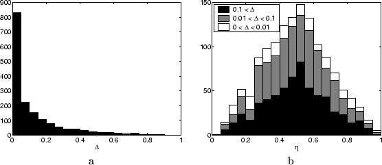
about 75 minutes. In Figure a we show a histograms of
the band widths (upper minus lower bound) found for the single node
marginals for all unclamped nodes.
Clearly, for the majority of the marginals very tight bounds are found.
converged in
about 75 minutes. In Figure a we show a histograms of
the band widths (upper minus lower bound) found for the single node
marginals for all unclamped nodes.
Clearly, for the majority of the marginals very tight bounds are found.
Although exact computations are infeasible for this network, one can
still use approximation methods to find an estimate of the single node
marginals. Therefore, we ran the cluster variation method (CVM)
as described in kappen02novel. For the clusters needed
by CVM, we simply took all node sets for which a potential
is defined. For every unclamped node we computed the relative position
of the approximation for the single node marginal within the bounding
interval, denoted by ![]() . Thus
. Thus ![]() indicates an approximation
equal to the lower bound, and similarly
indicates an approximation
equal to the lower bound, and similarly ![]() for the upper bound.
Although there is no obvious reason the approximated marginals should
be inside the bounding interval, it turned out they were. A histogram
of all the relative positions is shown in Figure b, where
we split up the full histogram into three parts, each referring to
a certain region of band widths. It is remarkable that the shape of
the histogram does not vary much given the tightness of the bounds.
Approximations tend to be in the middle, but for all band widths there
are approximations close to the edge.
for the upper bound.
Although there is no obvious reason the approximated marginals should
be inside the bounding interval, it turned out they were. A histogram
of all the relative positions is shown in Figure b, where
we split up the full histogram into three parts, each referring to
a certain region of band widths. It is remarkable that the shape of
the histogram does not vary much given the tightness of the bounds.
Approximations tend to be in the middle, but for all band widths there
are approximations close to the edge.
One can argue that we are comparing apples to pears, since we can
easily improve the results of both algorithms, while it is not clear
which cases are comparable. This is certainly true, but it is not our
intention to make a comparison to determine which method is the best.
Approximation and bounding methods both have their own benefits.
We presented Figure b to give at least some intuition about
the actual numbers. In general we found that approximations are usually
within the bounding intervals, when computation time is kept roughly
the same. This does, however, not make the bounds irrelevant. On the
contrary, one could use the bounding values as a validation whether
approximations are good or even use them as confidence intervals.