aDPCSP and solution

The resultant model space is translated into an aDCSP to enable the selection of a consistent set of assumptions, using advanced CSP solution techniques. The aDCSP derived from the above model space is depicted in Figure 12.

This aDCSP contains 11 attributes. They are listed with the corresponding assumption classes in table 4. The first 6 attributes correspond to the notion of relevance phenomenon: 3 population growth phenomena, 2 predation phenomena and 1 competition phenomenon to be precise. The other 5 attributes correspond to 5 sets of model types: 3 sets of population growth models and 2 sets of predation models.

Table 4: Attribute list

Attribute	Meaning
$x_{1}$	(relevant growth prey1)
$x_{2}$	(relevant growth prey2)
$x_{3}$	(relevant growth predator)
$x_{4}$	(relevant predation predator prey1)
$x_{5}$	(relevant predation predator prey2)
$x_{6}$	(relevant competition prey1 prey2)
$x_{7}$	(model size-1 *)
$x_{8}$	(model size-2 *)
$x_{9}$	(model size-3 *)
$x_{10}$	(model predation-phen-1 *)
$x_{11}$	(model predation-phen-2 *)

The assumptions from which the attributes were generated form domains of values. The resulting domains of the aforementioned attributes are summarised in table 5.

Table 5: The aDCSP for the 1 predator and 2 competing prey scenario: domains and their contents and meaning

Domain	Content	Meaning
$D_{1}$	$\{d_{1,y},d_{1,n}\}$	{population,none}
$D_{2}$	$\{d_{2,y},d_{2,n}\}$	{population,none}
$D_{3}$	$\{d_{3,y},d_{3,n}\}$	{population,none}
$D_{4}$	$\{d_{4,y},d_{4,n}\}$	{(population,population),none}
$D_{5}$	$\{d_{5,y},d_{5,n}\}$	{(population,population),none}
$D_{6}$	$\{d_{6,y},d_{6,n}\}$	{(population,population),none}
$D_{7}$	$\{d_{7,l},d_{7,e},d_{7,o}\}$	{logistic,exponential,other}
$D_{8}$	$\{d_{8,l},d_{8,e},d_{8,o}\}$	{logistic,exponential,other}
$D_{9}$	$\{d_{9,l},d_{9,e},d_{9,o}\}$	{logistic,exponential,other}
$D_{10}$	$\{d_{10,h},d_{10,lv}\}$	{Holling,Lotka-Volterra}
$D_{11}$	$\{d_{11,h},d_{11,lv}\}$	{Holling,Lotka-Volterra}

The activity constraints in the aDCSP describe the conditions that instantiate the subject of the assumptions that correspond to an attribute. Since each participant or relation has a label in the model space, a minimal set of assumptions under which it becomes part of the emerging model is available. When a participant or relation is the subject of an assumption, this label explicitly describes the sets of assumptions under which the attribute that corresponds to that subject should be activated. By translating the label of a subject into sets of attribute-value assignments, the antecedents of the activity constraints are constructed.

In this example, the relevance assumptions (attributes $x_1,\ldots,x_6$) take their subjects from the scenario, and hence, they are always active. The attributes related to the model assumptions for population growth are active if the corresponding assumptions denoting relevance of population growth are true. That is,

$$x_1:d_{1,y}\rightarrow (x_7)$$

$$x_2:d_{2,y}\rightarrow (x_8)$$

$$x_3:d_{3,y}\rightarrow (x_9)$$

The attributes related to the assumptions about the predation models are active if the corresponding assumptions denoting relevance of predation, and the assumptions describing relevance of population growth, are true for the populations involved in the predation relation. That is,

$$x_1:d_{1,y}\wedge x_3:d_{3,y}\wedge x_4:d_{4,y}\rightarrow (x_{10})$$

$$x_2:d_{2,y}\wedge x_3:d_{3,y}\wedge x_5:d_{5,y}\rightarrow (x_{11})$$

Figure 12 shows a graphical representation of these activity constraints.

Figure 12: aDCSP derived from the models space reflecting the 1 predator and 2 competing prey scenario

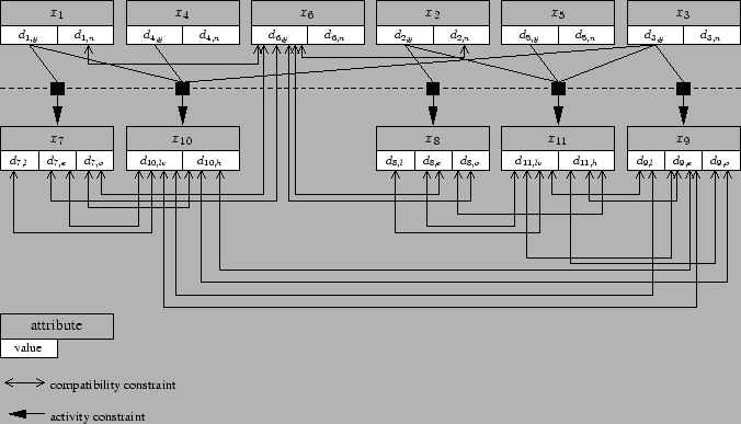
The compatibility constraints correspond directly to the inconsistencies in the nogood node. These inconsistencies have been discussed in the previous section and are depicted in Figure 12.

Once the aDCSP is constructed, preferences may be attached to attribute-value assignments. Suppose that preferences are only assigned to the standard population modelling choices, i.e. exponential growth, logistic growth, lotka-volterra predation and holling predation, and to the relevance of competition (because only one type model has been implemented for this phenomenon). For example, the following BPQs could be employed:

$$p_{\text{exponential}}<p_{\text{logistic}}$$

$$p_{\text{lotka-volterra}}<p_{\text{holling}}$$

$$p_{\text{competition}}$$

The logistic and Holling models are preferred over the exponential and Lotka-Volterra models because the former are generally regarded as being more accurate. Note that the preferences have been ordered in such a way that those corresponding to different phenomena are not related to one another. The justification for this ordering is that, even though the models are structurally connected (there are restrictions over which models can combined with one another), models of different phenomena inherently describe behaviours that can not be compared with one another. The preference assignments for attribute value assignments are summarised in table 6.

Table 6: Preference assignments for the 1 predator and 2 competing prey problem

Attribute	Preference assignments
$x_{1},\ldots,x_{5}$	no preference assignments
$x_{6}$	$P(x_{6}:d_{6,y})=p_{\text{competition}}$
$x_{7}$	$P(x_{7}:d_{7,l})=p_{\text{logistic}}$, $P(x_{7}:d_{7,e})=p_{\text{exponential}}$
$x_{8}$	$P(x_{8}:d_{8,l})=p_{\text{logistic}}$, $P(x_{8}:d_{8,e})=p_{\text{exponential}}$
$x_{9}$	$P(x_{9}:d_{9,l})=p_{\text{logistic}}$, $P(x_{9}:d_{9,e})=p_{\text{exponential}}$
$x_{10}$	$P(x_{10}:d_{10,h}=p_{\text{holling}}$, $P(x_{10}:d_{10,lv})=p_{\text{lotka-volterra}}$
$x_{11}$	$P(x_{11}:d_{11,h}=p_{\text{holling}}$, $P(x_{11}:d_{11,lv})=p_{\text{lotka-volterra}}$

Solving this aDPCSP is simple. First, the attributes $x_1,\ldots,x_6$ are activated. Each of these attributes is assigned $x_i:d_{i,y}$ because that assignment maximises the potential preference. Then, the attributes $x_7,\ldots,x_{11}$ are activated. Here, attributes $x_7,\ldots,x_9$ are assigned $x_i:d_{i,l}$ because the logistic growth model has the highest preference. Finally, $x_{10}$ and $x_{11}$ are assigned $x_{10}:d_{10,h}$ and $x_{11}:d_{11,h}$ because the Holling models have the highest preference and are not inconsistent with the logistic model committed earlier. 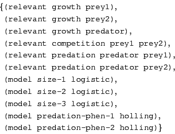The resulting solution satisfies the following set of assumptions:

$$\begin{split}\{&\texttt{(relevant growth prey1)},\\ &\texttt{... ...g)},\\ &\texttt{(model predation-phen-2 holling)}\} \end{split}$$