To take advantage of the potential cancellation of amplitude in nogoods described above we need a unitary mapping whose behavior is similar to the ideal mapping to supersets. There are two general ways to adjust the ideal mapping of sets to supersets (mixtures of these two approaches are possible as well). First, we can keep some amplitude at the same level of the lattice instead of moving all the amplitude up to the next level. This allows using the ideal map described above (with suitable normalization) and so gives excellent discrimination between solutions and nonsolutions, but unfortunately not much amplitude reaches solution level. This is not surprising: the use of random phases cancel the amplitude in nogoods but this doesn't add anything to solutions (because solutions are not a superset of any nogood and hence cannot receive any amplitude from them). Hence at best, even when all nogoods cancel completely, the amplitude in solutions will be no more than their relative number among complete sets, i.e., very small. Thus the random phases prevent much amplitude moving to nogoods high in the lattice, but instead of contributing to solutions this amplitude simply remains at lower levels of the lattice. Hence we have no better chance than random selection of finding a solution (but, when a solution is not found, instead of getting a nogood at the solution level, we are now likely to get a smaller set in the lattice). Thus we must arrange for amplitude taken from nogoods to contribute instead to the goods. This requires the map to take amplitude to sets other than just supersets, at least to some extent.
The second way to fix the nonunitary ideal map is to move amplitude
also to non-supersets. This can move all amplitude to the solution
level. It allows some canceled amplitude from nogoods to go to goods,
but also vice versa, resulting in less effective concentration into
solutions. This can be done with a unitary matrix as close as possible
to the nonunitary ideal map to supersets, and that also has a relatively
simple form. The general question here is given
k linearly independent vectors in
m dimensional space, with
![]() , find k
orthonormal vectors in the space as close as possible to the
k original ones. Restricting
attention to the subspace defined by the original vectors, this can be
obtained
, find k
orthonormal vectors in the space as close as possible to the
k original ones. Restricting
attention to the subspace defined by the original vectors, this can be
obtained![]() using the singular
value decomposition [24] (SVD) of the
matrix M whose columns are the
k given vectors. Specifically, this
decomposition is
using the singular
value decomposition [24] (SVD) of the
matrix M whose columns are the
k given vectors. Specifically, this
decomposition is ![]() , where
, where ![]() is a diagonal matrix containing the
singular values of M and both
is a diagonal matrix containing the
singular values of M and both
![]() and B have
orthonormal columns. For a real matrix
M, the matrices of the decomposition
are also real-valued. The matrix
and B have
orthonormal columns. For a real matrix
M, the matrices of the decomposition
are also real-valued. The matrix ![]() has orthonormal columns and is the closest set of
orthogonal vectors according to the Frobenius matrix norm. That is, this
choice for U minimizes
has orthonormal columns and is the closest set of
orthogonal vectors according to the Frobenius matrix norm. That is, this
choice for U minimizes
![]() among all unitary matrices. This construction fails
if
among all unitary matrices. This construction fails
if ![]() since an
m-dimensional space cannot have
more than m orthogonal vectors. Hence
we restrict consideration to mappings in the lattice at those levels
i where level
since an
m-dimensional space cannot have
more than m orthogonal vectors. Hence
we restrict consideration to mappings in the lattice at those levels
i where level ![]() has at least as many sets as level
i, i.e.,
has at least as many sets as level
i, i.e., ![]() . Obtaining a solution requires mapping up to level
L so, from
Eq. 1, this restricts
consideration to problems where
. Obtaining a solution requires mapping up to level
L so, from
Eq. 1, this restricts
consideration to problems where ![]() .
.
For example, the mapping from level 1 to 2 with ![]() given in Eq. 14
has the singular value decomposition
given in Eq. 14
has the singular value decomposition ![]() with this decomposition given explicitly as
with this decomposition given explicitly as

The closest unitary matrix is then
While this gives a set of orthonormal vectors close to the original
map, one might be concerned about the requirement to compute the SVD of
exponentially large matrices. Fortunately, however, the resulting
matrices have a particularly simple structure in that the entries depend
only on the overlap between the sets. Thus we can write the matrix
elements in the form ![]() (r is an
(i+1)-subset,
(r is an
(i+1)-subset, ![]() is an i-subset). The overlap
is an i-subset). The overlap ![]() ranges from i when
ranges from i when
![]() to 0 when there is no overlap. Thus instead of
exponentially many distinct values, there are only
to 0 when there is no overlap. Thus instead of
exponentially many distinct values, there are only ![]() , a linear number. This can be exploited to give a
simpler method for evaluating the entries of the matrix as
follows.
, a linear number. This can be exploited to give a
simpler method for evaluating the entries of the matrix as
follows.
We can get expressions for the a values for a given N and i since the resulting column vectors are orthonormal. Restricting attention to real values, this gives
where
is the number of ways to pick r with
the specified overlap. For the off-diagonal terms, suppose
![]() then, for real values of the matrix elements,
then, for real values of the matrix elements,
where
![]()
is the number of sets r with the
required overlaps with ![]() and
and ![]() , i.e.,
, i.e., ![]() and
and ![]() . In this sum, x is
the number of items the set r has in
common with both
. In this sum, x is
the number of items the set r has in
common with both ![]() and
and ![]() . Together these give
. Together these give ![]() equations for the values of
equations for the values of ![]() , which are readily solved
numerically
, which are readily solved
numerically![]() . There are
multiple solutions for this system of quadratic equations, each
representing a possible unitary mapping. But there is a unique one
closest to the ideal mapping to supersets, as given by the SVD. It is
this solution we use for the quantum search algorithm
. There are
multiple solutions for this system of quadratic equations, each
representing a possible unitary mapping. But there is a unique one
closest to the ideal mapping to supersets, as given by the SVD. It is
this solution we use for the quantum search algorithm![]() , although it is
possible some other solution, in conjunction with various choices of
phases, performs better. Note that the number of values and equations
grows only linearly with the level in the lattice, even though the
number of sets at each level grows exponentially. When necessary to
distinguish the values at different levels in the lattice, we use
, although it is
possible some other solution, in conjunction with various choices of
phases, performs better. Note that the number of values and equations
grows only linearly with the level in the lattice, even though the
number of sets at each level grows exponentially. When necessary to
distinguish the values at different levels in the lattice, we use
![]() to mean the value of
to mean the value of ![]() for the mapping from level
i to
for the mapping from level
i to ![]() .
.
The example of Eq. 14, with
![]() and
and ![]() , has
, has ![]() for Eq. 17 and
for Eq. 17 and
![]() for Eq. 19. The
solution of these unitarity conditions closest to
Eq. 14 is
for Eq. 19. The
solution of these unitarity conditions closest to
Eq. 14 is ![]() corresponding to Eq. 16.
corresponding to Eq. 16.
A normalized version of the ideal map has ![]() and all other values equal to zero. The actual values
for
and all other values equal to zero. The actual values
for ![]() are fairly close to this (confirming that the ideal
map is close to orthogonal already), and alternate in sign. To
illustrate their behavior, it is useful to consider the scaled values
are fairly close to this (confirming that the ideal
map is close to orthogonal already), and alternate in sign. To
illustrate their behavior, it is useful to consider the scaled values
![]() , with
, with ![]() evaluated using Eq. 18. The behavior of these values for
evaluated using Eq. 18. The behavior of these values for ![]() is shown in Fig. 2. Note that
is shown in Fig. 2. Note that ![]() is close to one, and decreases slightly as higher
levels in the lattice (i.e., larger i
values) are considered: the ideal mapping is closer to orthogonal at low
levels in the lattice.
is close to one, and decreases slightly as higher
levels in the lattice (i.e., larger i
values) are considered: the ideal mapping is closer to orthogonal at low
levels in the lattice.
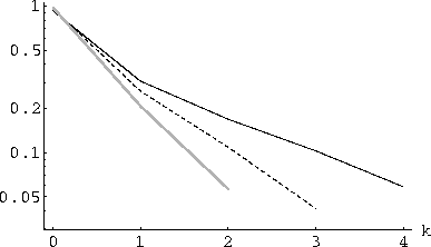
Figure 2: Behavior of ![]() vs. k on a log scale for N=10. The three curves show the values for i=4 (black), 3 (dashed) and 2 (gray).
vs. k on a log scale for N=10. The three curves show the values for i=4 (black), 3 (dashed) and 2 (gray).
Despite the simple values for the example of
Eq. 16, the ![]() values in general do not appear to have a simple
closed form expression. This is suggested by obtaining exact solutions
to Eqs. 17 and 19 using
the Mathematica symbolic algebra program [54]. In most cases this gives complicated
expressions involving nested roots. Since such expressions could
simplify, the
values in general do not appear to have a simple
closed form expression. This is suggested by obtaining exact solutions
to Eqs. 17 and 19 using
the Mathematica symbolic algebra program [54]. In most cases this gives complicated
expressions involving nested roots. Since such expressions could
simplify, the ![]() values were also checked for being close to rational
numbers and whether they are roots of single variable polynomials of low
degree
values were also checked for being close to rational
numbers and whether they are roots of single variable polynomials of low
degree![]() . Neither
simplification was found to apply.
. Neither
simplification was found to apply.
Finally we should note that this mapping only describes how the
sets at level i are mapped to the
next level. The full quantum system will also perform some mapping on
the remaining sets in the lattice. By changing the map at each step,
most of the other sets can simply be left unchanged, but there will need
to be a map of the sets at level ![]() other than the identity mapping to be orthogonal to
the map from level i. Any orthogonal
set mapping partly back to level i
and partly remaining in sets at level
other than the identity mapping to be orthogonal to
the map from level i. Any orthogonal
set mapping partly back to level i
and partly remaining in sets at level ![]() will be suitable for this: in our application there
is no amplitude at level
will be suitable for this: in our application there
is no amplitude at level ![]() when the map is used and hence it doesn't matter what
mapping is used. However, the choice of this part of the overall mapping
remains a degree of freedom that could perhaps be exploited to minimize
errors introduced by external noise.
when the map is used and hence it doesn't matter what
mapping is used. However, the choice of this part of the overall mapping
remains a degree of freedom that could perhaps be exploited to minimize
errors introduced by external noise.