An important question in the behavior of this search method is how
its average performance scales with problem size. To examine this
question, we consider the scaling with fixed ![]() . This is shown in
Figs. 7 and 8 for algorithms using random and inverted phases for
nogoods, respectively. To help identify the likely scaling, we show the
same results on both a log plot (where straight lines correspond to
exponential scaling) and a log-log plot (where straight lines correspond
to power-law or polynomial scaling).
. This is shown in
Figs. 7 and 8 for algorithms using random and inverted phases for
nogoods, respectively. To help identify the likely scaling, we show the
same results on both a log plot (where straight lines correspond to
exponential scaling) and a log-log plot (where straight lines correspond
to power-law or polynomial scaling).
It is difficult to make definite conclusions from these results for
two reasons. First, the variation in behavior of different problems
gives a statistical uncertainty to the estimates of the average values,
particularly for the larger sizes where fewer samples are available. The
standard errors in the estimates of the averages are indicated by the
error bars in the figures (though in most cases, the errors are smaller
than the size of the plotted points). Second, the scaling behavior could
change as larger cases are considered. With these caveats in mind, the
figures suggest that ![]() remains nearly constant for underconstrained
problems, even though the fraction of complete sets that are solutions
is decreasing exponentially. This behavior is also seen in the overlap
of the curves for small
remains nearly constant for underconstrained
problems, even though the fraction of complete sets that are solutions
is decreasing exponentially. This behavior is also seen in the overlap
of the curves for small ![]() in Figs. 4 and 5. For problems with more
constraints,
in Figs. 4 and 5. For problems with more
constraints, ![]() appears to decrease polynomially with the size of the
problem, i.e., the curves are closer to linear in the log-log plots than
in the log plots. This in confirmed quantitatively by making a least
squares fit to the values and seeing that the residuals of the fit to a
power-law are smaller than those for an exponential fit. An interesting
observation in comparing the two phase choices is that the scaling is
qualitatively similar, even though the phase inversion method performs
better. This suggests the detailed values of the phase choices are not
critical to the scaling behavior, and in particular high precision
evaluation of the phases is not required. Finally we should note that
this illustration of the average scaling leaves open the behavior for
the worst case instances.
appears to decrease polynomially with the size of the
problem, i.e., the curves are closer to linear in the log-log plots than
in the log plots. This in confirmed quantitatively by making a least
squares fit to the values and seeing that the residuals of the fit to a
power-law are smaller than those for an exponential fit. An interesting
observation in comparing the two phase choices is that the scaling is
qualitatively similar, even though the phase inversion method performs
better. This suggests the detailed values of the phase choices are not
critical to the scaling behavior, and in particular high precision
evaluation of the phases is not required. Finally we should note that
this illustration of the average scaling leaves open the behavior for
the worst case instances.

Figure 7: Scaling of the probability to find a solution using the random phase method, for ![]() of 1 (solid), 2 (dashed), 3 (gray) and 4 (dashed gray). This is shown on log and log-log scales (left and right plots, respectively).
of 1 (solid), 2 (dashed), 3 (gray) and 4 (dashed gray). This is shown on log and log-log scales (left and right plots, respectively).

Figure 8: Scaling of the probability to find a solution using the phase inversion method, for ![]() of 1 (solid), 2 (dashed), 3 (gray) and 4 (dashed gray). This is shown on log and log-log scales (left and right plots, respectively).
of 1 (solid), 2 (dashed), 3 (gray) and 4 (dashed gray). This is shown on log and log-log scales (left and right plots, respectively).
For the underconstrained cases in Figs. 7 and 8 there is a small additional difference between cases with an even and odd number of variables. This is due to oscillations in the amplitude in goods at each level of the lattice, and is discussed more fully in the context of SAT problems below.
Another scaling comparison is to see how much this algorithm
enhances the probability to find a solution beyond the simple quantum
algorithm of evaluating all the complete sets and then making a
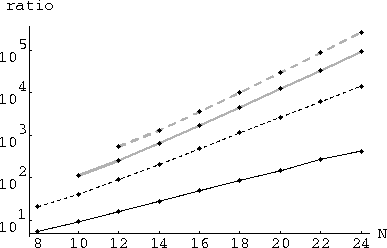
measurement. As shown in Fig. 9, this quantum algorithm appears to give an exponential improvement
in the concentration of amplitude into solutions. A more explicit view
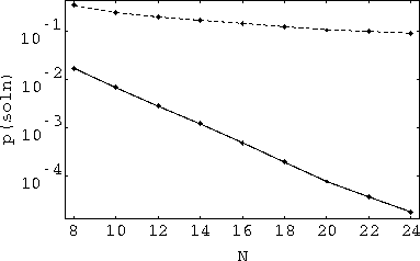
of this difference in behavior is shown in Fig. 10 for ![]() . In this figure, the dashed curve shows the behavior
of
. In this figure, the dashed curve shows the behavior
of ![]() for the phase inversion method, and is identical to
the
for the phase inversion method, and is identical to
the ![]() curve of Fig. 8.
curve of Fig. 8.

Figure 9: Scaling of the ratio of the probability to find a solution using the quantum algorithm to the probability to find a solution by random selection at the solution level, using the phase inversion method, for ![]() of 1 (solid), 2 (dashed), 3 (gray) and 4 (dashed gray). The curves are close to linear on this log scale indicating exponential improvement over the direct selection from among complete sets, with a higher enhancement for problems with more constraints.
of 1 (solid), 2 (dashed), 3 (gray) and 4 (dashed gray). The curves are close to linear on this log scale indicating exponential improvement over the direct selection from among complete sets, with a higher enhancement for problems with more constraints.

Figure 10: Comparison of scaling of probability to find a solution with the quantum algorithm using the phase inversion method (dashed curve) and by random selection at the solution level (solid curve) for ![]() equals 2.
equals 2.