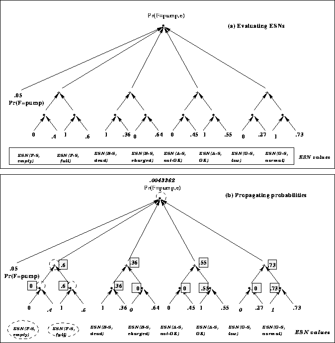
Now that we have a reduced Q-DAG, we can use it to compute answers to diagnostic queries. This section presents examples of this evaluation with respect to the generated Q-DAG.
Suppose that we obtain the readings dead, normal, ok and full for the battery, oil, alternator and fuel sensors, respectively. And let us compute the probability distribution over the fault variable. This obtained evidence is formalized as follows:
Suppose now that evidence has changed so that the value of fuel sensor is empty
instead of full. To update the probability assigned to node ![]() , a brute force method will re-evaluate the whole
Q-DAG. However, if a forward propagation scheme is used to implement the node
evaluator, then only four nodes need to be re-evaluated in
Figure 18(b) (those enclosed in circles) instead of thirteen (the
total number of nodes). We stress this point because this refined updating
scheme, which is easy to implement in this framework, is much harder to
achieve when one attempts to embed it in standard belief-network algorithms
based on message passing.
, a brute force method will re-evaluate the whole
Q-DAG. However, if a forward propagation scheme is used to implement the node
evaluator, then only four nodes need to be re-evaluated in
Figure 18(b) (those enclosed in circles) instead of thirteen (the
total number of nodes). We stress this point because this refined updating
scheme, which is easy to implement in this framework, is much harder to
achieve when one attempts to embed it in standard belief-network algorithms
based on message passing.

Figure: Evaluating the Q-DAG for the car diagnosis example given evidence
for sensors. The bar in (a) indicates the instantiation of the ESNs.
The shaded numbers in (b) indicate probability values that are computed by the
node evaluator. The circled operations on the left-hand-side of (b) are
the only ones that need to be updated if evidence for the fuel-system sensor
is altered, as denoted by the circled ESNs.