Neural Network Classifiers for Optical Chinese Character Recognition
Richard Romero, Robert Berger, Robert Thibadeau, and Dave Touretsky
Imaging Systems Lab, Robotics Institute
Carnegie Mellon University
5000 Forbes Avenue, Pittsburgh, PA 15213
Abstract
We describe a new, publicly accessible Chinese character recognition system based on a nearest neighbor classifier that uses several sophisticated techniques to improve its performance. To increase throughput, a 400-dimensional feature space is compressed through multiple discriminant analysis techniques to 100 dimensions. Recognition accuracy is improved by scaling these dimensions to achieve uniform variance. Two neural network classifiers are compared using the new feature space, Kohonen's Learning Vector Quantization and Geva and Sitte's Decision Surface Mapping. Experiments with a 37,000 character ground truthed dataset show performance comparable to other systems in the literature. We are now employing noise and distortion models to quantify the robustness of the recognizer on realistic page images.
1 Introduction
1.1 History of Chinese character recognition
Optical recognition of printed Chinese characters is a challenging problem that has been approached using a variety of techniques. Two of these are feature extraction and structural analysis [Suchenwirth et al. 89, Stallings 76, Zhang 87.] To date, though, no dominant method has emerged and the recognition rates being obtained are still far behind what has been achieved for texts in the Latin alphabet. The disparity in recognition rates is not due to lack of effort; the issues faced in each task are strikingly different.
Most recognition systems have dealt with only a limited set of fonts. The number of fonts in common use in modern Chinese texts is small, probably as a result of the large number of characters required. There are two main character sets in use today: simplified and traditional. The traditional set is larger and more elaborate, having evolved over hundreds of years. It is a complex system of pictograms, ideograms, phonograms, and phono-ideograms, generating about 12,000 entries in a relatively complete dictionary.(1) The complexity of a single character can be measured by the number of strokes it contains. In the Latin alphabet, characters contain from one to four strokes, while typical Chinese characters contain anywhere from one to 36 strokes.
From 1956 to 1964, the People's Republic of China introduced over 2,000 simplified characters. The effort was undertaken in order to reduce the number of strokes necessary to form the more common characters. A standard dictionary of the simplified character set contains about 7,000 of the characters in general use.
The People's Republic of China created the simplified standard for its own use. The traditional character set is still the norm in Taiwan, Hong Kong, Macau, and in overseas Chinese publications. Also in common use are four main font styles: songti, fangsongti, kaiti, and heiti. Examples of each are shown in Figure 1.1.
1.2 Problems faced
One of the first problems faced in building a Chinese OCR engine is the number of recognition classes. With about 7,000 characters in general use, it is necessary to build a system that can efficiently and reliably recognize far more classes than are required for Latin text. Furthermore, characters not represented in the original set may be encountered. In this paper, we will not consider the problem of characters not in the reference set.
FIGURE 1.1 Example characters in the four font styles. Left to right: songti, fangsongti, kaiti, and heiti.

A related problem is that the frequency of some characters is extremely low, measured in occurrences per million characters of text. In a frequency count over 1.8 million characters of Chinese text [Xiandai 86], 425 characters were encountered only once each, and the number of unique characters was only 4,574. Hence it is nearly impossible to build a corpus from actual scanned data that is large enough to contain all the characters that will ever be encountered, let alone obtain adequate statistical information on all characters.
We have created a set of ground truthed data containing over 55,000 characters from 111 scanned pages. Out of this, the largest segment uses the songti font and the simplified character set: 68 pages and 37,021 total characters, with 1850 unique characters. This paper will use the songti, simplified subset for reporting purposes.
1.3 Proposed solutions
The system we have built can be broken down into three stages: feature extraction, dimensionality reduction and scaling, and classification. The feature extraction stage decomposes a normalized image of the character into thirteen features of various sizes. This stage is detailed in the next section, describing what features are used and how they are calculated. The dimensionality reduction is done to increase the efficiency of classification. Dimension scaling improves the error rate of the classifier. This stage is described in Section 3. Section 4 describes the final classification step, done using a nearest neighbor approach in the newly reduced and scaled space. The dimension reduction and scaling as well as the classification steps require training data.
2 Character Features
2.1 The TECHIS feature set
The features that we used were originally developed by others also working on the Chinese character recognition problem. The most complete description of these features can be found in [Suchenwirth et al. 89], a study done by the Institutes of Measurement and Control Techniques, Communications, and Linguistics at the Technical University of Berlin. The project was named Teilautomatische Erkennung von chinesischer Schrift, or TECHIS, which translates as "part-automatic recognition of Chinese characters."
We aimed to replicate the features used by the TECHIS project in full. We extracted all of the features described in TECHIS, and attempted to utilize them all in an optimal manner. We will not attempt to either verify the use of any particular feature or fully describe all of the features here. A brief summary of the features and their sizes is given in Table 2.1.
2.2 Reference characters
TABLE 2.1 Brief summary of the features extracted.
-----------------------------------------------------------------
Name                                                   Dimensions
-----------------------------------------------------------------
Blackness (number of black pixels)                     1
Stroke Width                                           1
Total Stroke Length                                    1
Horizontal Projection                                  64
Vertical Projection                                    64
Number of Horizontal Transitions (white-to-black)      1
Number of Vertical Transitions (white-to-black)        1
First Order Peripheral Features                        32
Second Order Peripheral Features                       32
Stroke Density at (fig) and (fig)                      16
Local Direction Contributivity with four regions and   64
four directions
Maximum Local Direction Contributivity                 64
Stroke Proportion                                      32
Black Jump Distribution in Balanced Subvectors         32
Total Feature Dimensions                              405

-----------------------------------------------------------------
The original database of characters was generated from the songti TrueType font distributed in the Apple Chinese Language Kit. The set consisted of 6,992 characters, including the Latin alphabet, Arabic numerals, and standard symbols. The TrueType font was used to generate standardized bitmaps, such that the largest of the characters fit inside a 64 x 64 bitmap. During the course of testing our classifier, we discovered that two of the characters in the songti font distributed with the Apple Chinese Language Kit were incorrectly drawn.
The images were rescaled so that they were centered and filled a 64 x 64 bitmap. If the aspect ratio was greater than 1.6, the aspect ratio was preserved and the X and Y axes were scaled using the same factor. If the aspect ratio was less than 1.6, the image was expanded using different scales for X and Y axes so that both width and height were scaled up to 64. The image scaling was done in a simple linear fashion as described in [Suchenwirth et al. 89].
Once all of the scaling had been done, features were extracted. The total number of feature dimensions was 405
3 Feature Transformation
3.1 The TECHIS distance measure
The TECHIS project employed an ad hoc mixture of statistics and heuristics to obtain a distance measure between reference characters and test data. Through experimentation and analysis, it was found that by using a combination of the first order peripheral features, second order peripheral features, stroke density, and the black jump distribution in balanced subvectors, the effect any single type of noise had on the recognition rates was minimized. The reason for this, the authors explain, is that these particular types of features are generally uncorrelated and affected by different types of noise.
In order to combine these four multidimensional features into a single distance value, a distance was first calculated for each feature, then those four distances were combined. The distance computation uses a simple linear distance measure, the  norm:
norm:
(EQ 1) 
Simply put, the distance between the feature vector x and the prototype feature value for class i is the sum of the absolute differences of all vector elements. The next reduction, from four feature distances to a single distance, was done as:
(EQ 2) 
where  is the distance from feature j in class i, and N is the number of classes. This is then called the relative distance, since it is measuring distance from class i relative to the distance from all other classes. Using this method of feature combination, an impressive 99.92% recognition rate on test data of over 20,000 characters was reported. However, after implementing the same features and distance measures, we obtained only a 92% recognition rate on our 58,482 character database.
The justification for these equations was partially based on a supposed failure of statistical methods to properly deal with multiple types of multidimensional features. However, we have implemented statistical methods to both combine the different features in a beneficial manner and reduce the number of dimensions. Then, instead of computing a simple linear distance, the true Euclidean distance measure can be utilized.
3.2 Dimension reduction transformation
What follows is a brief review of multiple discriminant analysis. For a complete discussion, see [Duda and Hart 73]. One assumption made, which is not explicit in the derivation, is that the within-class variances are homogeneous. In other words, a single type of noise affects a feature in a consistent way, regardless of the character. Now, with  being the set of exemplars in class i and x being the entire feature vector for that particular exemplar, the scatter matrix for class i can be defined as,
(EQ 3) 
with
(EQ 4) 
and the total within-class scatter matrix is
(EQ 5)  .
.
The between-class scatter matrix is defined as
(EQ 6)  ,
,
where m is the overall mean, and it can be shown that
(EQ 7) 
where  is the total scatter matrix. The scatter matrices are analogous to covariance matrices. What we wish to compute is W , a transformation matrix that maximizes the new between-class scatter,
  , with respect to the new within-class scatter,
  . Then, using W , we can define the following:
(EQ 8) 
(EQ 9) 
(EQ 10) 
(EQ 11) 
(EQ 12) 
It follows, then, that
(EQ 13) 
(EQ 14) 
One way to then maximize the between-class scatter with respect to the within-class scatter is to use the determinants of the scatter matrices as an overall measure of variance. The determinant is the same as the product of the eigenvalues, and this corresponds directly with the product of the variances. So, we wish to minimize
(EQ 15)  .
.
The solution to the matrix W , can be shown to correspond to the generalized eigenvectors corresponding to the largest eigenvalues in
(EQ 16) 
where the  are the columns of W . To reduce the original space of d dimensions, the size of the x vectors, to a c dimensional space, take the eigenvectors corresponding to the c largest eigenvalues to form W .
With the nearest-neighbor based classifiers described in section 4 it is desirable to scale the transformed features so they have equal within-class variances, resulting in hyperspherical class distributions. In order to scale the transformed feature axes, we need an estimate for the variance in dimension i . This can be found from Equation 13, since we know the form for  . The variance in dimension i is then
(EQ 17)  , with
  as column i of W .
And the transformation matrix can be scaled by replacing each  with
with
(EQ 18) 
thereby scaling each new dimension by a factor of its new standard deviation.
3.3 Scatter matrix computation
In order to compute the two scatter matrices, our ground truth data in the simplified songti character set was used. First, all the features were calculated for all of the characters. For any character class that had 10 or more exemplars, the corresponding feature vectors were included in  . From this set of feature vectors, the scatter matrix computations were computed directly from the above equations.
Out of a set of 37,021 character exemplars, there were 681 unique characters with 10 or more exemplars, and a total of 33,531 characters. Out of this reduced set of characters, the mean number of occurrences was 49.2, the median 27, and the maximum 1,524.
The reason for not including characters with fewer exemplars is that their statistical validity is questionable in terms of how much they should contribute to the overall within-class variance. The more exemplars available, the more stable the estimate for  , which implies that the calculations for
  ,
,  , and
, and  are more stable.
4 Neural Network Classifiers
Both neural classification schemes that we used are essentially nearest-neighbor prototype matching. The difference between the two lies solely in the training algorithms that are used to determine the prototypes.
4.1 The LVQ algorithm
LVQ (Learning Vector Quantization) was developed by [Kohonen 88] as a method of vector classification. Using a fixed number of class prototypes, LVQ proceeds as follows: find the nearest prototype to the current exemplar. If the prototype and exemplar are from the same class, move the prototype closer to the exemplar. If they are from different classes, move the prototype away from the exemplar. The direction of movement is defined by the line joining the two vectors.
The LVQ algorithm adjusts the prototypes to approximate the density of exemplars in each class. If exemplars are uniformly distributed, the prototypes will uniformly fill the class boundaries. In our application, each class is represented by a single prototype. The resulting distribution of prototypes is such that they are approximately located at the mean of all exemplars.
4.2 The DSM algorithm
The DSM (Decision Surface Mapping) algorithm [Geva and Sitte 91] is a refinement of the LVQ algorithm. Geva and Sitte showed that fewer classification errors result if prototypes are concentrated close to the class boundaries, no matter what the actual distribution of training instances. This mapping of the decision surface is what the DSM algorithm tries to achieve.
For each incorrectly classified training instance, the DSM algorithm moves the nearest prototype slightly away from the training instance, as in LVQ. It also finds the nearest prototype with the correct label and moves that one slightly closer to the training instance. For correctly classified training instances the DSM algorithm does nothing. Thus, prototypes that are located well in the interior of a class are untouched by the DSM algorithm. Those located less centrally are moved by both intra- and extra-class exemplars until they lie right on the class boundary.
DSM can be unstable when there is noise in the training set. In that case, Geva and Sitte suggest that LVQ might be preferable. But in our application, where the initial prototypes are drawn from noise-free PostScript fonts and the training set has been carefully ground truthed, our experiments show that our modified version of DSM retains its stability.
4.3 Dynamic node addition
Our variant of the DSM algorithm allows for the creation of new prototypes, based on the distance to the closest prototype relative to the closest correct prototype, when classification fails. If the ratio of these distances exceeds a threshold, a new prototype will be created, positioned at the location of the incorrectly classified exemplar. This procedure allows us to start the system out with a minimal set of just 7000 prototypes (one per class), and grow it automatically as needed to insure that the shapes of decision boundaries are well represented.
4.4 Training parameters and data
Given that we have exemplar E which is of class  , and the closest prototype is of class
  , we can define
  as the distance from E to
  , and
, and  as the distance from E to
  . If
. If  , then the DSM algorithm will first check that
  , where y is the threshold for adding new prototypes. If
  is true, then
  is moved a distance
  towards
  , and
, and  is moved a distance
  away from
  . We define
  , where
  is the current epoch of training. The available training parameters, then, are
  ,
,  , and
, and  .
.
For the LVQ algorithm, if  is in the same class as
  , we move
  towards
  a distance
  , with
  defined as before. If
  is not in the same class as
  , we move
  away from
  the same distance
  . The training parameters for LVQ are
  and
and  .
.
5 Recognition Results
5.1 Results before training
Before the DSM or LVQ classifier training, multiple discriminant analysis was used to transform the features extracted from the TrueType songti font. At this point, the dimension of the new space can be set, using as a gauge the percentage of total variance explained by those dimensions. To measure this, we sum the eigenvalues corresponding to the eigenvectors which make up the transform matrix. The ratio of this sum to the sum of all the eigenvalues is roughly the percentage of variance still present in the new space. Based on these measures, we estimated that approximately 90% of the variance could be described in a space of 100 dimensions.(2) As explained above, each dimension individually is the linear transform defined by an eigenvector. So, the eigenvectors of the 100 largest eigenvalues were used.
In order to verify that 100 dimensions was a reasonable number, we tested our ground truthed characters using three dimension sizes. The results are shown in Table 5.1 for the 37,021 songti characters.
TABLE 5.1 Results of using different numbers of dimensions for data
		transformation.
------------------------------------------
Dimensions  Correct  Incorrect  Hit Rate %
------------------------------------------
 50         35,240   1781       95.19
100         35,568   1453       96.08
150         35,355   1666       95.50

------------------------------------------
It may seem surprising that using 150 dimensions resulted in worse performance than using 100, but this is probably due to an over-fitting of the problem. By including those extra 50 dimensions, we are almost surely adding more noise than actual information. On the other hand, using just 50 dimensions appears to omit some useful information. So, 100 dimensions appears to be a good approximation to the optimal number.
5.2 Results after training
Differences in training parameters were found to have little effect on recognition rates. For example, in one set of training runs, three values of y were used to determine the threshold for adding new prototypes for the DSM algorithm: 1.5, 1.75, and 2.0. The differences in the resulting recognition rates were found to be less than 0.03%. This is comparable to differences seen between separate runs using the same parameter settings, and is attributed to the random presentation of training examples producing slightly different modifications of the prototypes.
Reasonable values for the DSM parameters were  ,
,  , and
, and  . Using these settings, it took from 5 to 12 epochs to learn to classify the entire training set without error. The number of prototypes added was between 3 and 8. Thus, almost all the classes were sufficiently compact and well-separated in the transformed feature space that only a single prototype was required.
For the LVQ algorithm, values of  and
and  were found to be more suitable. The LVQ algorithm in all instances ran for 50 epochs without converging to a perfect fit of the training data, making the DSM algorithm much faster in terms of training epochs. For the three training set sizes of 6,761, 10,894, and 17,588 characters, recognition rates on the actual training sets were 99.78%, 99.72%, and 99.64%, respectively.
TABLE 5.2.a Summary of results with different training and test set sizes.
-----------------------------------------------------------------------------------------------------------------------
Number of   Number of    Number of   Number of   Characters              Hit Rate %  Characters              Hit Rate %
Training    Unique       Test        Unique       Correct                             Correct
Characters  Characters   Characters  Test
                                     Characters
-----------------------------------------------------------------------------------------------------------------------
 6,761      1,103        30,260      1,706       29,631                  97.92       29,821                  98.55
10,894      1,249        26,127      1,673       25,660                  98.21       25,790                  98.71
17,588      1,541        19,433      1,485       19,135                  98.47       19,204                  98.82

-----------------------------------------------------------------------------------------------------------------------
TABLE 5.2.b Summary of results with different training sets and identical test
		sets.
----------------------------------------------------------------------------------
Number of   Characters              Hit Rate %  Characters              Hit Rate %
Training    Correct                             Correct
Characters
----------------------------------------------------------------------------------
 6,761      14,519                  97.70       14,631                  98.45
10,894      14,584                  98.14       14,669                  98.71
17,588      14,625                  98.41       14,679                  98.78
----------------------------------------------------------------------------------
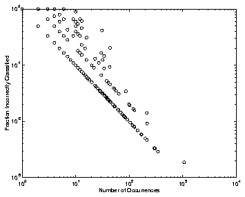
FIGURE 5.3.b Log scale plot of character frequency versus error rate using DSM.

Table 5.2.a shows a summary of the results using different training set sizes. In this table, the test set consisted of all the characters which had not been used in training. In Table TABLE 5.2.b, the same three training sets are shown, but a common set of test data is used. It contains 14,861 characters, 1,354 of which are unique. In all of these results, only the training and test set sizes are varied; the learning parameters remain constant.
5.3 Conclusions
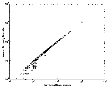
FIGURE 5.3.a Log scale plot of character frequency versus number of instances correctly classified using DSM.

In Figure 5.3.a and 5.3.b, two views of the same information are given. Both of these plots show that the frequency of occurrence of a character has a strong correlation with its recognition rate. (In both plots, characters that were recognized without error have been omitted(3).) In evaluating a Chinese character recognition engine, this correlation is one which we believe to be useful. It shows that the characters with low recognition rates tend to be those occurring with low frequency. While acceptable for Chinese character recognition, this sort of correlation is not desired at all in Latin character recognition, simply because there are only a handful of characters, each of which is frequent in comparison to a Chinese character. Similar plots are found using the LVQ algorithm.
In comparing the LVQ to the DSM training algorithm, it appears that the data is not best separated by modeling decision boundaries, but rather the distribution centers. It does appear, however, that LVQ and DSM may converge to the same placement of class prototypes as the training set size increases.
Using the DSM algorithm, consider the case where a class has a single prototype and very few exemplars. Furthermore, assume that classes in general are uniformly distributed in their locations, and normally distributed in their shapes. The final location of the prototype under DSM is largely constrained by the convex hull of the exemplars, which is made up of the data outliers. With a small number of exemplars, there is no reason to believe that the mean of the outliers will accurately predict a mean for the class. As the number of exemplars increases, the outliers should come closer to forming a hyper-ellipse centered at the true mean of the class's distribution.
If the class is not distributed normally in shape, or if classes are not, in general, uniformly distributed in the transformed feature space, it is unclear which algorithm would yield the better answer. It does appear that being able to dynamically add prototypes is desirable, as the LVQ algorithm never found a perfect solution for the training data given a single prototype per class. This is evidence that at least some classes are either not well separated or not normally distributed.
6 Future Work
6.1 Additional features
Because of the image normalization, some Chinese characters become nearly impossible to distinguish. One obvious way to correct this is to include the aspect ratio as a feature. Another possible solution is to use the same scaling factor for the two axes, so that the aspect ratio is preserved in the normalized image. A problem with both of these approaches is that within a single font family, different global aspect ratios can be used. Manipulating the aspect ratio is easily accomplished with scalable fonts such as TrueType and PostScript.
An alternative approach is to compute either the average or maximum height and width for a section of text. Then, compute each individual character's width and height relative to the average or maximum. The easiest way to isolate a section of text is to use the current row. Using the entire page is not advisable, as titles and headings are almost always done in a size larger than the body.
6.2 Noise and distortion models
One of the biggest problems encountered when training a recognition engine for Chinese characters is obtaining adequate amounts of training data, since many characters are encountered only rarely.. Our method was to start with the Apple Chinese Language Kit TrueType fonts for our initial prototypes, and then introduce actual scanned images which had been hand-labeled.(4) This is obviously a time consuming and expensive endeavor, which gives only modest returns. Currently, we are exploring the possible use of noise and distortion models to enlarge the dataset. The idea is to find distortion models that show similar characteristics to real data acquired by scanning. It is hoped that by using such models we can increase the effectiveness of the multiple discriminant analysis and the generalization obtained during neural network training.
References
Duda, Richard; Hart, Peter: Pattern Classification and Scene Analysis 1973, 114-121. New York: John Wiley & Sons.
Geva, Shlomo; Sitte, Joaquin: Adaptive Nearest Neighbor Pattern Classification, IEEE Transactions on Neural Networks, 1991, Vol. 2, No. 2.
Kohonen, Teuvo: Self-organization and Associative Memory, 2nd ed., 1988, 199-202.
Stallings, William: Approaches to Chinese Character Recognition. Pattern Recognition 1976, Vol. 8, 87-98.
Suchenwirth, Richard; Guo, Jun; Hartmann, Irmfried; Hincha, Georg; Krause, Manfred; Zhang, Zheng: Optical Recognition of Chinese Characters. Advances in Control Systems and Signal Processing 1989, Vol. 8. Braunschweig: Friedr. Vieweg & Sohn.
Xiandai Hanyu Pinlu Cidian: Frequency Dictionary of the Modern Chinese Language. Languages Institute Press 1986.
Zhang, Zheng: A Structural Analysis Method for Constrained Handprinted Chinese Character Recognition. Journal of the Beijing Institute of Technology 1987.1, 1-7.
Appendix A: Image Samples
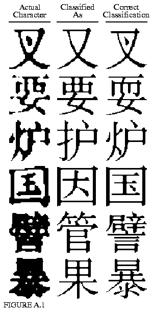
Figure A.1 shows some of the incorrectly classified characters. On the next page, in Figures A.2 and A.3, are portions of two of the testpages used, magnified 1.5 times.

FIGURE A.2
FIGURE A.3
Appendix B: FTP Instructions
A demonstration version of our system is available via anonymous FTP. To retrieve it, open a connection to host ftp.cs.cmu.edu (128.2.206.173) and log in as user anonymous. with userid@host as the password. Then cd to /afs/cs/project/pcvision/ChineseOCR. Note: you must cd directly to this directory; the parent directories will not be accessible to anonymous FTP users. Remember to select image (binary) mode before retrieving compressed or executable files.<
There are subdirectories for document images, fonts, and the demo application, presently a SunOS 4.x SPARC executable. Versions for other platforms may be provided at a later date. A full description of the directory's organization can be found in the README file.
Footnotes
- (1)
- The actual number of dictionary entries for the traditional character set is measured in the tens of thousands, as many words can be formed through the compounding of simpler words. But many of the characters are used so rarely that dictionaries commonly omit them.
- (2)
- The reason for the qualifiers "approximately" and "roughly" is the problems we encountered with floating point imprecision. The scatter matrix was ill-conditioned for finding eigenvalues and eigenvectors, and several of the eigenvalues were very close to zero.
- (3)
- In FigureFIGURE 5.3.a, the characters recognized without error are of the form , since the number correct is the number present. In FigureFIGURE 5.3.b, these same characters have a miss rate of 0, and their log becomes .
- (4)
- We used a standard coding scheme known as the GB code, analogous to ASCII. Unfortunately, GB codes are only defined for the simplified character set. For the traditional character set, an encoding called Big 5 was used.

 norm:
norm:


 being the set of exemplars in class i and x being the entire feature vector for that particular exemplar, the scatter matrix for class i can be defined as,


 . From this set of feature vectors, the scatter matrix computations were computed directly from the above equations.


 , and the closest prototype is of class
  , we can define
  as the distance from E to
  , and
, and  as the distance from E to
  . If
. If  , then the DSM algorithm will first check that
  , where y is the threshold for adding new prototypes. If
  is true, then
  is moved a distance
  towards
  , and
, and  is moved a distance
  away from
  . We define
  , where
  is the current epoch of training. The available training parameters, then, are
  ,
,  , and
, and  .
. is in the same class as
  , we move
  towards
  a distance
  , with
  defined as before. If
  is not in the same class as
  , we move
  away from
  the same distance
  . The training parameters for LVQ are
  and
and  .
. ,
,  , and
, and  . Using these settings, it took from 5 to 12 epochs to learn to classify the entire training set without error. The number of prototypes added was between 3 and 8. Thus, almost all the classes were sufficiently compact and well-separated in the transformed feature space that only a single prototype was required.

