shape optimization
Read an extended abstract about this work.
Find below some of the results for model problems we have tested in one and two spatial dimensions.
shape matching problem
 In the shape matching problem we try to match a target shape starting
from an arbitrary initial configuration. We formulate this problem as
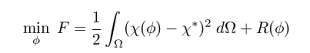
an unconstrained minimization problem where the objective functional is
the misfit F between the current and target shapes. X and X*
are their corresponding continuous Heavisides/characteristic
functionals shown in F. A regularization term R is
needed to render the solution unique. Tikhonov and
Total Variation are options we consider. We also
regularize against a signed distance like function but this is
primarily used on PDE constrained problems.
In the shape matching problem we try to match a target shape starting
from an arbitrary initial configuration. We formulate this problem as
an unconstrained minimization problem where the objective functional is
the misfit F between the current and target shapes. X and X*
are their corresponding continuous Heavisides/characteristic
functionals shown in F. A regularization term R is
needed to render the solution unique. Tikhonov and
Total Variation are options we consider. We also
regularize against a signed distance like function but this is
primarily used on PDE constrained problems.
This model somehow resembles the Mumford-Shah model used in image segmentation. We tried it using Tikhonov regularization and segmented MRI brain images, our first attempt at variational image processing. Our results are promising. We need to add noisy though to make it more realistic and apply TV.
Test cases of shape matching follow below. Click on image to play an animation in Quicktime format.
1D examples
quicktime animation 253K
(128 elements)

The shape match on a line is the problem of equalizing segment lengths.
The animation shows the level set function evolution during the
iterations of the nonlinear solver. We use boxes to visualize segments
and when they align the matching is absolute. The orange box on the
animation is the non-zero part of the binary Heaviside when applied to
the evolving level set function which is plotted as an orange
curve. The target segment is shown as a blue box. For visualisation
purposes only, its height is twice the orange one. An iteration counter is
shown on the top right corner. In this example, we started with a
parabola and it took the solver 12 iterations to find an optimal
solution. Observe the topology change from one to two segments. Used
Tikhonov regularization.
2D examples
quicktime movie 632K
(256 x 256 mesh).
short quicktime 291K
(128 x 128 mesh)
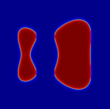
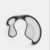
We are matching against two kidney beans in the plane. Continuous
Heavisides, as opposed to binary Heavisides in the previous example,
are plotted and projected onto the zero plane. This is an old, outdated
example where we used a pure Newton step and did not apply continuation
on the regularization parameter. We like to keep this example for
reference reasons (and because it is a nice movie to show on
presentations!). The final result is still a very good match but
obtained at a much higher price than, for example, the example shown
below for the same geometry. In this case, we started the level set
function as a sphere. The solver took around 30 iterations (we could
have stopped at 12 or so since there was no further improvement on the
misfit after that point but we imposed the stop criterion to be the
Lagrangian gradient). Used Tikhonov regularization.
quicktime movie 787K
(64 x 64 mesh)
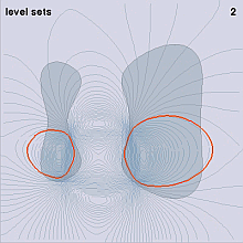
We have in this example the same kidney beans but the solver has been
considerably improved. It took only 12 iterations for our
Gauss-Newton-Krylov solver to obtain a perfectly matching result. Note
that the shape is very close to the target after 4 or 5 iterations. The
remaining iterations serve to capture the very fine details not seen by
the naked eye (!) and to stabilize the regularization. The level set
curves are plotted on the plane together with the evolving interface
and target beans.
We started with a signed distance function and it deforms to something
else (observe the non equidistant level curves at the end). Check the
3D animation below. Employed Tikhonov regularization.
quicktime movie 511K
(64 x 64 mesh)
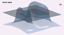
A 3D view of the evolution of the level sets for the example shown
above.
Copyright Alexandre Cunha
updated on jul/2004