PbR is inspired by the local search techniques used in combinatorial optimization. An instance of a combinatorial optimization problem consists of a set of feasible solutions and a cost function over the solutions. The problem consists in finding a solution with the optimal cost among all feasible solutions. Generally the problems addressed are computationally intractable, thus approximation algorithms have to be used. One class of approximation algorithms that have been surprisingly successful in spite of their simplicity are local search methods [1,64].
Local search is based on the concept of a neighborhood. A neighborhood of a solution p is a set of solutions that are in some sense close to p, for example because they can be easily computed from p or because they share a significant amount of structure with p. The neighborhood generating function may, or may not, be able to generate the optimal solution. When the neighborhood function can generate the global optima, starting from any initial feasible point, it is called exact [64, page 10].
Local search can be seen as a walk on a directed graph whose vertices are solutions points and whose arcs connect neighboring points. The neighborhood generating function determines the properties of this graph. In particular, if the graph is disconnected, then the neighborhood is not exact since there exist feasible points that would lead to local optima but not the global optima. In PbR the points are solution plans and the neighbors of a plan are the plans generated by the application of a set of declarative plan rewriting rules.
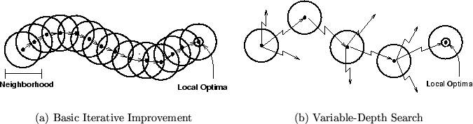
The basic version of local search is iterative improvement. Iterative improvement starts with an initial solution and searches a neighborhood of the solution for a lower cost solution. If such a solution is found, it replaces the current solution and the search continues. Otherwise, the algorithm returns a locally optimal solution. Figure 5(a) shows a graphical depiction of basic iterative improvement. There are several variations of this basic algorithm. First improvement generates the neighborhood incrementally and selects the first solution of better cost than the current one. Best improvement generates the complete neighborhood and selects the best solution within this neighborhood.
Basic iterative improvement obtains local optima, not necessarily the global optimum. One way to improve the quality of the solution is to restart the search from several initial points and choose the best of the local optima reached from them. More advanced algorithms, such as variable-depth search, simulated annealing and tabu search, attempt to minimize the probability of being stuck in a low-quality local optimum.
Variable-depth search is based on applying a sequence of steps as opposed to only one step at each iteration. Moreover, the length of the sequence may change from iteration to iteration. In this way the system overcomes small cost increases if eventually they lead to strong cost reductions. Figure 5(b) shows a graphical depiction of variable-depth search.
Simulated annealing [45] selects the next point randomly. If a lower cost solution is chosen, it is selected. If a solution of a higher cost is chosen, it is still selected with some probability. This probability is decreased as the algorithm progresses (analogously to the temperature in physical annealing). The function that governs the behavior of the acceptance probability is called the cooling schedule. It can be proven that simulated annealing converges asymptotically to the optimal solution. Unfortunately, such convergence requires exponential time. So, in practice, simulated annealing is used with faster cooling schedules (not guaranteed to converge to the optimal) and thus it behaves like an approximation algorithm.
Tabu search [36] can also accept cost-increasing neighbors. The next solution is a randomly chosen legal neighbor even if its cost is worse than the current solution. A neighbor is legal if it is not in a limited-size tabu list. The dynamically updated tabu list prevents some solution points from being considered for some period of time. The intuition is that if we decide to consider a solution of a higher cost at least it should lie in an unexplored part of the space. This mechanism forces the exploration of the solution space out of local minima.
Finally, we should stress that the appeal of local search relies on its simplicity and good average-case behavior. As could be expected, there are a number of negative worst-case results. For example, in the traveling salesman problem it is known that exact neighborhoods, that do not depend on the problem instance, must have exponential size [71]. Moreover, an improving move in these neighborhoods cannot be found in polynomial time unless P = NP [63]. Nevertheless, the best approximation algorithm for the traveling salesman problem is a local search algorithm [40].