Experiments

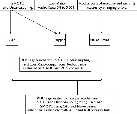
We used three different machine learning algorithms for our experiments. Figure 6 provides an overview of our experiments.

  

Figure 6: Experiments Overview

1.

C4.5: We compared various combinations of SMOTE and under-sampling with plain under-sampling using C4.5 release 8 [21] as the base classifier.

2.

Ripper: We compared various combinations of SMOTE and under-sampling with plain under-sampling using Ripper [22] as the base classifier. We also varied Ripper's loss ratio [31,4] from 0.9 to 0.001 (as a means of varying misclassification cost) and compared the effect of this variation with the combination of SMOTE and under-sampling. By reducing the loss ratio from 0.9 to 0.001 we were able to build a set of rules for the minority class.

3.

Naive Bayes Classifier: The Naive Bayes Classifier can be made cost-sensitive by varying the priors of the minority class. We varied the priors of the minority class from 1 to 50 times the majority class and compared with C4.5's SMOTE and under-sampling combination.

These different learning algorithms allowed SMOTE to be compared to some methods that can handle misclassification costs directly. %FP and %TP were averaged over 10-fold cross-validation runs for each of the data combinations. The minority class examples were over-sampled by calculating the five nearest neighbors and generating synthetic examples. The AUC was calculated using the trapezoidal rule. We extrapolated an extra point of TP = 100% and FP = 100% for each ROC curve. We also computed the ROC convex hull to identify the optimal classifiers, as the points lying on the hull are potentially optimal classifiers [1].