Abstract
Recognizing landmark is a critical task for mobile robots. Landmarks are used for robot positioning, and for building maps of unknown environments. In this context, the traditional recognition techniques based on strong geometric models cannot be used. Rather, models of landmarks must be built from observations using image-based techniques. This paper addresses the issue of building image-based landmark descriptions from sequences of images and of recognizing them. Beyond its application to mobile robot navigation, this approach addresses the more general problem of identifying groups of images with common attributes in sequences of images. We show that, with the appropriate domain constraints and image descriptions, this can be done using efficient algorithms.
Starting with a "training" sequence of images, we identify groups of images corresponding to distinctive landmarks. Each group is described by a set of feature distributions. At run-time, the observed images are compared with the sets of models in order to recognize the landmarks in the input stream. Domain constraints are used in order to reduce the search space, both in creating the models and in recognizing them. Geometrical constraints include the orientation of the camera with respect to the direction of travel. Temporal constraints include the use of the vehicle position associated with each image in order to derive clusters of images that are spatially consistent temporally.
We conducted experiments by using sequences of images in both urban and natural environments. Results show that small sets of landmarks can be extracted from training sequences and that those landmarks can be recognized in test sequences.
Introduction
Recognizing landmarks in sequences of images is a challenging problem for a number of reasons. First of all, the appearance of any given landmark varies substantially from on observation to the next. In addition to variation due to different aspects, illumination change, external clutter, and changing geometry of the imaging devices are other factors affecting the variability of the observed landmarks. Finally, it is typically difficult to use accurate 3D information in landmark recognition applications. For those reasons, it is not possible to use many of the object recognition techniques based on strong geometric models.
The alternative is to use image-based techniques in which landmarks are represented by collection of images which are supposed to capture the "typical" appearance of the object. The information most relevant to recognition is extracted from the collection of raw images and used as the model for recognition. This process is often referred to as "visual learning".
Progress has been made recently in developing such approaches. For example, in object modeling See P. Gros, O. Bournez and E. Boyer. Using Local Planar Geometric Invariants to Match and Model Images of Line Segments. To appear in Int. J. of Computer Vision and Image Understanding. , 2D or 3D model of objects are built for recognition applications. An object model is built by extracting features from a collection of observations. The most significant features are extracted for the entire set and are used in the model representation. Extension to generic object recognition were presented recently See S. Carlsson. Combinatorial Geometry for Shape Representation and Indexing. Proc. International Workshop on Object Representation for ComputerVision. Cambridge, England, April 1996. .
Other recent approaches use the images directly to extract a small set of characteristic images of the objects which are compared with observed views at recognition time. For example, the eigen-images techniques are based on this idea.
Those approaches are typically used for building models of single object observed in isolation. In the case of landmark recognition for navigation, there is no practical way to isolate the object in order to build models. Worse, it is often not known in advance which of the objects observed in the environment would constitute good landmarks. Visual learning must therefore be able to identify groups of images corresponding to "interesting" landmarks and to construct models amenable to recognition out of raw sequences of images.
A similar problem, although in a completely different context, is encountered in image indexing, where the main problem is to store and organize images to facilitate their retrieval See B.Lamiroy and P.Gros. Rapid Object Indexing and Recognition Using Enhanced Geometric Hashing. Proc. of the 4th European Conf. on Computer Vision, Cambridge, England, pages 59--70, vol. 1, April 1996. See C. Schmid and R. Mohr. Combining Greyvalue Invariants with Local Constraints for Object Recognition. Proceedings of the Conference on Computer Vision and Pattern Recognition, San Francisco, California, USA. pages 872--877, June 1996 . The emphasis in this case is the kind of features used and the type of requests that can be made by the user. For image retrieval, actual systems (QBIC, JACOB, Virage...) are closer to smart browsing than to image recognition. Using criteria such as color, shape, regions, etc., the systems search for images most similar to a given image. The user can then interact with the system to define which of these images seem the most interesting for him, and a new set of closer images is displayed.
Our system tries to combine these two categories of systems. In a training stage, the system is given a set of images in sequence. The aim of the training is to organize these images into groups based on similarity of feature distributions between images. The size of the groups obtained may be defined by the user, or by the system itself. In the latter case, the system tries to finds the most relevant groups, taking the global distribution of the images into account. In a second step, the system is given new images, which it tries to classify as one of the learned groups, or in the category of unrecognized images.
The basic representation is based on distributions of different feature characteristics. All these different kinds of histograms are computed for the whole image and for a set of sub-images. Tests similar to Chi-square tests are used to compare these histograms and define a distance between images. This distance is then used to cluster the images in what are called groups. An agglomerative grouping algorithm is used at this stage. At each step of the algorithm, the clusters made are evaluated by an entropy-like function, whose maximum gives the optimal solution in a sense specified later. Each group is then characterized by a set of feature histograms. When new images are given to the system, it evaluates a distance between these images and the groups. The system determines to which group this image is the closest, and a set of thresholds is used to decide if the image belongs to this group.
The main goal of the work presented here was to explore the use of tools and methods in the field of image retrieval to the problem of landmark recognition. It is clear that the global architecture of the system is close to that of object recognition systems See P. Gros, O. Bournez and E. Boyer. Using Local Planar Geometric Invariants to Match and Model Images of Line Segments. To appear in Int. J. of Computer Vision and Image Understanding. : a training stage in which 3D shape, 2D aspects, or groups, are characterized is followed by a recognition stage in which this information is used to recognize the models, objects or groups in new images. The difference comes from the wide diversity of the images and from the groups which are not reduced to a single aspect of an object. The two challenging tasks which we concentrate on in the remainder of the paper are to define these groups more precisely as sets of images, and to learn automatically a characterization for each group: what remains invariants, what varies and in which proportions.
The first section of the paper deals with the feature distributions, their computation and their comparison. The second section addresses the computation and the characterization of groups. The third section concerns the classification of new images according to the groups previously defined. Experimental data and results are presented in the fourth section.
Representing Images
In this section, we give a brief overview of the features used for representing images. Since an individual feature can be characteristic of an aspect of an object, but probably fails to characterize well a set of aspects, we use a statistical description of a large number of features as our basic representation Representing Feature Distributions
Five basic features are currently used: distributions of normalized color and intensity, edges, segments, and parallel segments. Additional features can be added as needed. The basic image representation is a set of feature distributions.
Edges are computed using Deriche's edge detector See R. Deriche Using Canny's Criteria to Derive a Recursively Implemented Optimal Edge Detector. Int. Journal of Computer Vision 1(2), pages 167--187, 1987 . Segments are computed as a polygonal approximation of the edges See R. Horaud, T. Skordas and F. Veillon. Finding Geometric and Relational Structures in An Image Proc. of the 4th European Conf. on Computer Vision, Antibes, France pages 374--384, April 1990 . Parallel segments are pairs of segments having approximately the same direction and facing one another.
Among the characteristics computed from these five features are: color and grey levels; edge density, orientation, length and position; segment density, orientation, length, and position; parallel segment density, orientation, length, and position, and, finally, the angles between adjacent segments.
Feature densities are computed in two ways: first as the ratio of the number of features (edges, segments and parallel segments, respectively) to the area of the image or sub-image concerned; second as the ratio of the sum of all the feature lengths to the area of the image or sub-image.
All the other measurements are computed and the results stored in histograms. Each bucket of the length histograms indicates how many features a length has in a given interval. (The size of this interval was chosen to be equal to 10 pixels.) The same is done for the orientations and angles, with buckets of 5 degrees. In the case of edges, the orientation is computed at each pixel of each edge, and can have only eight different values. The position gives rise to a 2D histogram, each bucket indicating the total length of the features present in a sub-image of size 20 pixels by 20 pixels. The color and grey level histograms have buckets of size 5.
The number of features (pixels, segments, edges...) is associated with each histogram, such that the latter can be interpreted in terms of relative numbers (e.g., the proportion of segments which have a length between 10 and 20 pixels).
The position of a particular object in an image may vary substantially between observations. Therefore, it is important to build the representation in a way that allows for different placements of the object with similar resulting feature distributions. This is done by subdividing the image into smaller chunks, in which the feature distributions are computed. All these histograms and densities, except those relative to feature position, are computed for the whole image and for the sub-images obtained by dividing the image by 4, then 9, and then 16. The position histograms are computed only for the global image, i.e., 90 densities and 333 histograms are computed to characterize each image.
Comparing Feature Distributions
The feature distributions from two images are compared using a distance similar to the chi-square distance. This distance, in its simplest form, evaluates the probability that two sets of data, here the histograms or the densities, are derived from the same theoretical distribution. If the distributions are h = (hi) and l = (li), their difference is computed as See W.H. Press, S.A. Teukolsky, W.T. Vetterling and B.P. Flannery. Numerical Recipes in C. Second Edition, Cambridge University Press 1992. : d(h, l) = Si(hi - li)2/(hi + li).
The main problem is to derive a global distance between two images from the individual distances computed for each type of density and histogram. The distance dij between two images i and j is defined as the linear combination of the distances between individual feature distributions: dij = Sk lk d(h, l), where the sum is taken over all the feature distributions used for representing the images.
When nothing is known about the distributions and their range of variation, all the weights can be taken equal to one. This simple approach gives good results in practice, but a better approach is to compute the weights based on the relative scales of the feature distributions. For each kind of density or histogram, the distance between every pair of images is computed, and the variance s2k of these distances is derived. The coefficient relative to this particular distribution can be chosen as lk = 1/s2k. This choice of weights has the effect of normalizing the distributions and of assigning the same relative importance to all the partial distances used.
As soon as more information is known about the relevance of the different histograms and densities, the weights can be updated. For example, with our data, densities are usually less relevant than the histograms. Uniform weights, although they may appear limited, give good results, because distances between densities are smaller than that between histograms. Once initial groups are computed based on a set of weights, the weights can be updated by requiring that images belonging to a group be closer to that group than to any other. Essentially, this adjustment stage enhances the discrimination among groups.
From Images to Landmarks
Given a sequence of images, we now want distinctive landmarks, that is, we want to split the sequence into groups of images, and find a characterization of each of these groups which allows further classification.
This step is difficult to do fully automatically in general. The main reason is that there is not a task-independent definition of the type of image groups that are needed. Our approach is to use task constraints to guide the grouping process. Specifically, given an initial grouping of images, we select groups based on three constraints. First, only the groups that contain a large enough number of images from different aspects are retained. Second, groups that do not provide significant discrimination are discarded. This is important to ensure that, at recognition time, only the groups that can be easily distinguished are used as models. Finally, the recorded sensor position for each training image is used for ensuring that the groups are spatially coherent.
Computing Initial Image Groups
Once the distance matrix is computed, a simple agglomerative method is used to split the image set into initial groups. First each image is put in a different group. Then the two closest groups are grouped and the distance matrix is updated. Finally, the algorithm iterates the previous step until an ending condition is verified.
Let |L| denote the number of elements of the image group L. The update of the matrix consists of suppressing the two lines and two columns i and j corresponding to the groups I and J which are grouped, and then adding a new line and column for the new group formed. The diagonal term of the new line added is:
(|I|(|I|-1)dii+|J|(|J|-1)djj+2|I||J|dij)/(|I|(|I|-1)+|J|(|J|-1) +2|I||J|)
The non diagonal term corresponding to the new group and a group k is:

These formulas show that, at each iteration, the only information needed is the distance matrix and the number of elements in each group. Each term of the matrix is thus the mean distance between the images of two groups, or the mean distance of the images of a same group.
Controlling the Grouping Algorithm
The grouping algorithm described above is general. In particular, it does not incorporate a control structure that stops the grouping process when groups of images corresponding to recognizable landmark are formed. An automatic method was developed for controlling image grouping.
Given a set of image groups, let us denote the distance matrix by (dij) and the number of images of the group i by ni. If the images used to learn the groups form a representative sample, and if they are spread nearly uniformly in representation space, the probability that an unknown image will be classified in the group i (pi) or in no group at all (p0) can be evaluated. If n denotes the number of groups:

These formulas state that the probability pi that a new image belongs to a group is proportional to the size dii of this group, and that the probability p0 of being in no group is proportional to the distances djk between the groups. The factor 2/(n-1) is used to compensate the number of non-diagonal terms of the distance matrix with respect to the number of diagonal terms.
In the case where the images are known not to have a uniform distribution in a region of their representation space, this can be taken into account by using these other formulas:
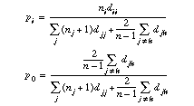
In these new formulas, not only the size of the groups is taken into account but also their density, which is proportional to ni. The probability p0 is also a function of the size of the groups: for the same distances between the groups, the smaller the groups, the bigger their density, and the smaller is the probability of having a new image between them.
The evaluation function is the entropy associated with this set of probabilities S= -Si pi ln pi, and the process is stopped when this entropy is maximal. This maximizes the information provided to the user by each classification request.
