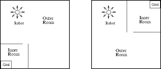
Figure 5: The Old Task
In the previous section, the existing task and the new task were strongly related, the walls and doorways were fixed and only the goal position was different. In this section, no such relationship is assumed. The robot is faced with a brand new task and must determine what, if any, relationship exists between the new task and any previous tasks.

The experimental testbed is again a simulated robot environment, but this time the problem is simplified to just an inner rectangular room and an outer L-shaped room. Figures 5 and 6 show two possible room configurations. Again, the thin lines are the walls of the room, the thick lines the boundary of the state space. Suppose the robot had already learned a function for the ``Old Task'' of Figure 5. We would hope that we could adapt the old solution to fit the closely related ``New task'' of Figure 6.
The steps, in this example, are essentially those in the previous one. But now as the learning process is started afresh, there are no features and the system must wait until they emerge through the normal reinforcement learning process. Then we can proceed much as before. First a graph for the inner room is extracted. The best matching graph in the case base from the old task is rotated and stretched to fit the new task. Next a matching graph for the outer L-shaped room is rotated and stretched around the larger inner room. The same transforms are then applied to the associated functions, any height adjustments carried out and the functions composed to form an approximate solution to the new task.
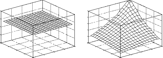
In this example, the first step in the process is to locate the goal. As there is no partition to aid the search, the initial value function is set to a mid-range constant value (see Figure 7). This allows some limited learning which encourages the system to move away from regions it has explored previously, to prevent a completely random walk through state space. Once the goal is located, the learning algorithm is reinitialized with a function for the same goal position but no walls (see Figure 8). If such a function does not exist in the case base, any rough approximation could be used instead. The ``no walls'' function is not used exactly as stored in the case base. The difference between the goal and the rest of the state space is reduced by scaling the function then adding a constant. This reduces the ``bias'' of the function, allowing the learning algorithm to alter it relatively easily as new information becomes available.

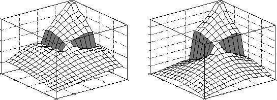
Figure 9 shows the resultant function about 3000 exploratory steps from the beginning of the learning process. Again, the large gradients associated with the walls are readily apparent. Figure 10 shows the function for the new task if it had been allowed to converge to a good solution. Both functions have roughly the same form, the large gradients are in the same position, although learning the latter took some 200,000 steps. After the ``no walls'' function is introduced the features take some time to clearly emerge. The snake will typically filter out features that are too small and not well formed. Additional filtering at the graphical level further constrains acceptable features. The total set of features must produce a consistent composite graph, the doorways from different subgraphs must align and the graph must overlay the complete state space. There must also be a matching case in the case base for every subtask. Many of these checks and balances will be removed when the iterative updating technique of Section 6.2 is incorporated.
