Representation of OMPs

Technically, OMPs are combinations of so-called basic preference quantities (BPQs), which are the primitive units of preference or utility valuation associated with possible design decisions. Because it is often difficult to evaluate these BPQs numerically, they are ordered relative to one another employing similar ordering relations as those employed by relative order-of-magnitude calculi [5,6].

Figure 1: Sample space of BPQs

Let $\mathds{B}$ be the set of all BPQs with respect to a particular decision problem. The BPQs in $\mathds{B}$ are ordered with respect to one another at two levels of granularity, by two relations $\ll$ and $<$. First, $\mathds{B}$ is partitioned into orders of magnitude, which are ordered by $\ll$. Then, the BPQs within each order of magnitude are ordered by $<$. Formally, an order-of-magnitude ordering over BPQs $\mathds{B}$ is a tuple $\langle \mathbf{O},\ll\rangle$, where $\mathbf{O}=\{O_1,\ldots,O_q\}$ is a partition of $\mathds{B}$ and $\ll$ is an irreflexive and transitive binary relation over $\mathbf{O}$. Any subset of BPQs $O\in\mathbf{O}$ is said to be an order of magnitude in $\mathds{B}$. Similarly, a within-magnitude ordering over a set of BPQs is a tuple $\langle O,<\rangle$, where $O$ is an order of magnitude in $\mathds{B}$ and $<$ is an irreflexive and transitive binary relation over $O$.

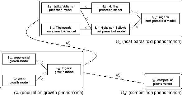
To illustrate these ideas, consider the problem of constructing an ecological model describing a scenario containing a number of populations. Let some of the populations be parasites and others be hosts for these parasites. Also, assume that certain populations compete with others for scarce resources. In order to construct a scenario model, the compositional modeller must make a number of model design decisions: which population growth, host-parasitoid and competition phenomena are relevant, and which types of model best describe these phenomena.

Figure 1 shows a sample space of BPQs that correspond to the selection of types of model. For the sake of illustration, the presumption is made that the quality of a scenario model depends on the inclusion of types of model, rather than on the inclusion or exclusion of phenomena. Apart from $b_{23}$ and $b_{31}$, all BPQs correspond to standard textbook ecological models¹. BPQ $b_{23}$ stands for the use of a population growth model that is implicit in another population growth model (the Lotka-Volterra model, for instance, implicitly includes its own concept of growth). Finally, BPQ $b_{31}$ is the preference associated with a competition model (say, the only one included in the knowledge base).

The 9 BPQs in this sample space are partitioned over 3 orders of magnitude. The $\ll$ relation orders the orders of magnitude: $O_2\ll O_1$ and $O_2\ll O_3$. The binary $<$ relation orders individual BPQs within an order of magnitude. In the BPQ ordering within $O_1$, for instance, Rogers' host-parasitoid model ($b_{11}$) is preferred over that by Nicholson and Bailey ($b_{12}$) and the Holling predation model ($b_{13}$). The latter two models can not be compared with one another, but they both are preferred over the Lotka-Volterra model. Furthermore, Thompson's host-parasitoid model is less preferred than that of Nicholson and Bailey, but it can not be compared with the Lotka-Volterra and Holling models.