EC distribution

The purpose of this section is twofold: to provide a detailed characterization of the EC distribution, and to discuss a narrowed-down subset of the EC distributions with only five free parameters ($\lambda_Y$ is fixed) which we will use in our moment matching algorithms. Both results are summarized in Theorem 3.

To motivate the theorem in this section, suppose one is trying to match the first three moments of a given distribution, $G$, to a distribution, $P$, which is the convolution of exponential distributions (possibly with different rates) and a two-phase Coxian$^+$ PH distribution. If $G$ has sufficiently high second and third moments, then a two-phase Coxian$^+$ PH distribution alone suffices and we need no exponential distributions (recall Theorem 2). If the variability of $G$ is lower, however, we might try appending an exponential distribution to the two-phase Coxian$^+$ PH distribution. If that does not suffice, we might append two exponential distributions to the two-phase Coxian$^+$ PH distribution. Thus, if $G$ has very low variability, we might be forced to use many phases to get the variability of $P$ to be low enough. Therefore, to minimize the number of phases in $P$, it seems desirable to choose the rates of the exponential distributions so that the overall variability of $P$ is minimized. One could express the appending of each exponential distribution as a ``function'' whose goal is to reduce the variability of $P$ yet further.

Definition 12   Let $X$ be an arbitrary distribution. Function $\phi$ maps $X$ to $\phi(X)$ such that $\phi(X)=Y\ast X$, the convolution of $Y$ and $X$, where $Y$ is an exponential distribution whose rate, $\lambda_Y$, is chosen so that the normalized second moment of $\phi(X)$ is minimized. Also, $\phi^i(X)=\phi(\phi^{i-1}(X))$ refers to the distribution obtained by applying function $\phi$ to $\phi^{i-1}(X)$ for integers $i\geq 1$, where $\phi^0(X)=X$.

Observe that, when $X$ is a $k$-phase PH distribution, $\phi^N(X)$ is a $(k+N)$-phase PH distribution.

In theory, function $\phi$ allows each successive exponential distribution which is appended to have a different rate. Surprisingly, however, the following theorem shows that if the exponential distribution ${Y}$ being appended by function $\phi$ is chosen so as to minimize the normalized second moment of $\phi(X)$ (as specified by the definition), then the rate of each successive $Y$ is always the same and is defined by the simple formula shown in the theorem below. The theorem also characterizes the normalized moments of $\phi^i(X)$.

Theorem 3   Let $\phi^i(X) = {Y_i} \ast \phi^{i-1}(X)$, and let $\lambda_{Y_i}$ be the rate of the exponential distribution $Y_i$ for $i=1,...,N$. Then,

$$\lambda_{Y_i} = \frac{1}{(m_2^{X}-1)\mu_1^{X}}$$ (2.1)

for $i=1,...,N$. The normalized moments of $Z_N = \phi^N(X)$ are:

$$\begin{eqnarray*} m_2^{Z_N} & = & \frac{(m_2^{X}-1)(N+1)+1}{(m_2^{X}-1)N+1} \\ ... ...}{\left((m_2^{X}-1)(N+1)+1\right)\left((m_2^{X}-1)N+1\right)^2}. \end{eqnarray*}$$

Proof:We first characterize ${Z} = \phi({X}) = {Y} \ast {X}$, where ${X}$ is an arbitrary distribution with a finite third moment and ${Y}$ is an exponential distribution. The normalized second moment of ${Z}$ is

$$m_2^{Z} = \frac{m_2^{X}+2y+2y^2}{(1+y)^2},$$

where $y = \mu_1^{Y} / \mu_1^{X}$. Observe that $m_2^{Z}$ is minimized when $y=m_2^{X}-1$, namely when

$$\mu_1^{Y} = (m_2^{X} - 1)\mu_1^{X}.$$ (2.2)

Observe that when $\mu_1^Y$ is set at this value, the normalized moments of ${Z}$ satisfy:

$$m_2^{Z} = 2 - \frac{1}{m_2^{X}} \quad\mbox{and}\quad m_3^{Z}... ...1}{m_2^{X}(2m_2^{X}-1)}m_3^{X} + \frac{3(m_2^{X}-1)}{m_2^{X}}.$$

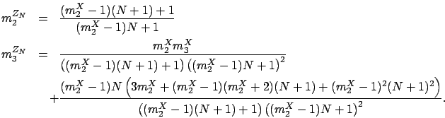
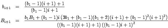
We next characterize ${Z_i} = \phi^i({X}) = Y_i \ast \phi^{i-1}({X})$ for $2\leq i\leq N$. By the above expression on $m_2^Z$ and $m_3^Z$, the second part of the theorem on the normalized moments of $Z_N$ follow from solving the following recurrence equations (where we use $b_i$ to denote $m_2^{\phi^i({X})}$ and $B_i$ to denote $m_3^{\phi^i({X})}$):

$$b_{i+1} = 2 - \frac{1}{b_i} \quad\mbox{and}\quad B_{i+1} = \frac{B_i}{b_i(2b_i-1)}+\frac{3(b_i-1)}{b_i}.$$

The solutions for these recurrence equations are

$$\begin{eqnarray*} b_{i+1} & = & \frac{(b_1-1)(i+1)+1}{(b_1-1)i+1}\\ B_{i+1} & =... ...^2\right)}{\left((b_1-1)(i+1)+1\right)\left((b_1-1)i+1\right)^2} \end{eqnarray*}$$

for all $i\geq 0$. These solutions can be verified by substitution. This completes the proof of the second part of the theorem.

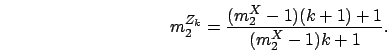
The first part of the theorem on $\lambda_{Y_i}$ is proved by induction. When $i=1$, (2.1) follows from (2.2). Assume that (2.1) holds for $i=1,...,k$. Let ${Z_k}=\phi^k({X})$. By the second part of the theorem, which is proved above,

$$m_2^{Z_k} = \frac{(m_2^{X}-1)(k + 1) +1}{(m_2^{X}-1)k+1}.$$

Thus, by (2.2),

$$\frac{1}{\lambda_{Y_{k+1}}} = \mu_1^{{Y}_{k+1}} = (m_2^{Z_k}-1)\mu_1^{Z_k} = (m_2^{X}-1)\mu_1^{X}.$$

    width 1ex height 1ex depth 0pt

Corollary 1   If $X$ is in set $\left\{F\mid 2 < m_2^F\right\}$, then ${Z}=\phi^N({X})$ is in set $\left\{F\mid \frac{N+2}{N+1} < m_2^F < \frac{N+1}{N}\right\}$.

Proof:By Theorem 3, $m_2^{Z}$ is a continuous and monotonically increasing function of $m_2^{X}$. Thus, the infimum and the supremum of $m_2^{Z}$ are given by evaluating $m_2^{Z}$ at the infimum and the supremum, respectively, of $m_2^{X}$. When $m_2^{X} \rightarrow 2$, $m_2^{Z} \rightarrow \frac{N+2}{N+1}$. When $m_2^{X} \rightarrow\infty$, $m_2^{Z} \rightarrow \frac{N+1}{N}$.     width 1ex height 1ex depth 0pt

Corollary 1 suggests the number, $N$, of times that function $\phi$ must be applied to ${X}$ to bring $m_2^{Z}$ into a desired range, given the value of $m_2^{X}$.