


Next: Analysis of the FB
Up: Dimensionality reduction
Previous: Dimensionality reduction
Contents
Analysis of the birth-and-death FB process
In this section, we analyze a simplest FB process shown in Figure 3.13.
Our goal is to reduce the FB process (2D Markov chain)
to a QBD process with a finite number of phases (1D Markov chain)
which closely approximates the FB process.
Figure 3.23:
An analysis of the FB process in
Figure 3.13 via DR. (a) The background process in
Figure 3.13(a) is approximated by a Markov chain on a finite state space.
(c) The FB process in
Figure 3.13(c) is approximated by a 1D Markov chain.
(a) Approximate background process
(b) Foreground process when the background process is in level  |
|
Observe that the infinite number of phases in the FB process
stems from the infinite number of states in the background
process,  (Figure 3.13(a)). This motivates us to
approximate by a Markov chain with a finite number of states,
(Figure 3.13(a)). This motivates us to
approximate by a Markov chain with a finite number of states,
 (Figure 3.23(a)). In process , all the states in levels
  of process is
aggregated into two states labeled . That is, the sojourn
time in levels ,
of process is
aggregated into two states labeled . That is, the sojourn
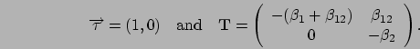
time in levels ,  , is approximated by a two-phase PH
distribution (as defined in Section 2.2) with parameters:
, is approximated by a two-phase PH
distribution (as defined in Section 2.2) with parameters:
We use the moment matching algorithm developed in Chapter 2
to choose the parameters of the PH distribution so that
the first three moments of are matched.
The sojourn time is exactly the same
as the busy period in an M/M/1 queue where the arrival rate is  and the service rate is
  . Thus, the first three moments of are
where
 .
The following theorem implies that two phases are sufficient to match
these three moments by a PH distribution.
.
The following theorem implies that two phases are sufficient to match
these three moments by a PH distribution.
Theorem 8
Let denote the duration of an M/GI/1 busy period where service demand  has
an arbitrary distribution with finite third moment and where the
job starting the busy period has size
has
an arbitrary distribution with finite third moment and where the
job starting the busy period has size  whose distribution is in
 (recall Definition 7 in Section 2.1).
Then, the distribution of is in
.
(recall Definition 7 in Section 2.1).
Then, the distribution of is in
.
A proof of Theorem 8 is postponed to Appendix A.
Theorem 8 is useful in determining the sufficient number
of phases in a PH distribution to well-represent a busy period duration
without explicitly computing the moments of the busy period.
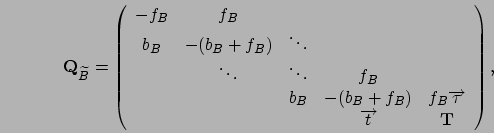
By replacing the background process by , the 2D Markov
chain (Figure 3.13(c)) is reduced to a 1D Markov chain shown
in Figure 3.23(c). More formally,
the 1D Markov chain is a QBD process, and its generator matrix,  , is obtained via the generator
matrix of ,
, is obtained via the generator
matrix of ,
 , as follows.
First, observe that
, as follows.
First, observe that
where
 .
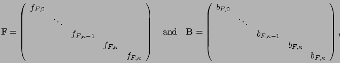
Generator matrix is then given by
.
Generator matrix is then given by
where  and
and  are
are
 diagonal matrices,
 ,
and
,
and
 .
.
In general, the stationary probabilities in the 1D Markov chain can
immediately be translated into the stationary probabilities in the foreground process. On the other hand, the stationary probabilities
in the background process needs to be analyzed independently, since
its state space is aggregated in the 1D Markov chain. Observe,
however, that the background process is easy to analyze, since it is
simply a birth-and-death process without dependency on the foreground process.
Next: Analysis of the FB
Up: Dimensionality reduction
Previous: Dimensionality reduction
Contents
Takayuki Osogami
2005-07-19

![\includegraphics[width=\linewidth]{fig/MC/background-DR.eps}](img795.png)
![\includegraphics[width=.85\linewidth]{fig/MC/foreground.eps}](img796.png)
![\includegraphics[width=\linewidth]{fig/MC/RFBQBD-DR.eps}](img797.png)