Scenario + Knowledge Base = Model Space

As previously stated, the aim of a compositional modeller is to translate a scenario into a scenario model. Both are representations of the system of interest though they model the system at a different level of detail. The knowledge base provides the foundation for translation. All the scenario models that can be constructed from the given scenario, with regard to the knowledge base, are stored in the model space.

A model space is an ATMS [7] containing all the participants, relations and assumptions that can be instantiated from a given scenario. In this work, the generalised version of the ATMS, as introduced by de Kleer [8], is employed as it allows the use of negations of nodes in the justifications. The algorithm $\CALL{generateModelSpace}{\langle O,R\rangle}$ describes how such a model space can be created from a scenario $\langle O,R\rangle$. It first initialises the model space $\theta$ with the participant instances ($O$) and the relation instances ($R$) from the scenario. Then, for each model fragment whose source-participants and structural conditions match participants and relations already in $\theta$, new instances of its target-participants, assumptions and postconditions are added to $\theta$. Because each property definition $\langle P^s,\Phi,\pi\rangle$ is equivalent to a model fragment $\langle P^s,\{\},\Phi,\{\pi\},\{\},\{\} \rangle$, this procedure applies to property definitions as well as model fragments. Matching the source-participants and structural conditions of a model fragment $\mu$ to the emerging model space is performed by the function match$(\mu,\theta,\sigma)$ as specified below, where $\mu$ is the model fragment being matched, and $\sigma$ is a substitution from the source-participants of $\mu$ to participant instances.

$$(\mu,\theta,\sigma)= \begin{cases}\text{true} & \text{if } \quad\... ...n\Phi^s(\mu), \sigma\phi\in\theta\\ \text{false} & \text{otherwise} \end{cases}$$

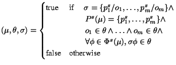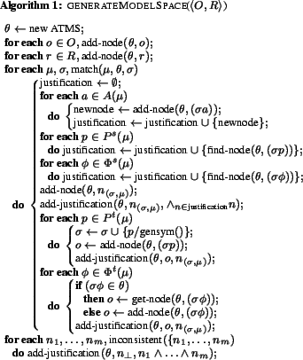
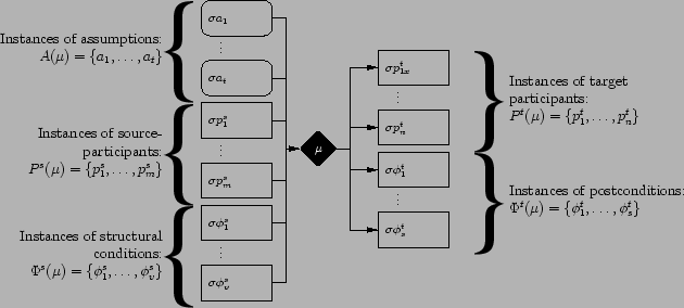
Figure 5: Model fragment application

Each match, specified by a model fragment $\mu$ and a substitution $\sigma$, is processed as follows:

• For each assumption $a\in A(\mu)$, a new node, denoting the assumption instance $\sigma a$, is created and added to $\theta$.
• Then, a new node $n_{(\sigma,\mu)}$, denoting the instantiation of $\mu$ via substitution $\sigma$, is created, added to $\theta$ and justified by the implication:

  $$(\wedge_{a\in A(\mu)}\sigma a)\wedge(\wedge_{p\in P^s(\mu)}\sigma p)\wedge(\wedge_{\phi\in \Phi^s(\mu)}\sigma \phi)\rightarrow n_{(\sigma,\mu)}$$

  
  

• Finally, a new instance for each target-participant $p\in P^t(\mu)$ and for each postcondition $\phi\in\Phi^t(\mu)$, provided $\sigma\phi$ does not already exist in the model space $\theta$, is created. For the target-participants, this involves creating a new symbol for each new participant instance with the function gensym$()$ and extending $\sigma$ with the substitution $\{p/$gensym$()\}$. A new node $n$ is created and added to $\theta$ for each new participant instance $\sigma p$ and for each new instantiated relation $\sigma\phi$. Each of these nodes is justified by the implication $n_{(\sigma,\mu)}\rightarrow n$.

To illustrate this procedure, Figure 5 shows a graphical representation of the inferences that are constructed by applying a model fragment $\mu=\langle P^s,P^t,\Phi^s,\Phi^t,A,\{\}\rangle$ with respect to a substitution $\sigma$.

Figure 6: Sources of inconsistency

Once all possible applications of model fragments have been exhausted, the inconsistencies in the model space are identified and recorded in the ATMS. In the algorithm, nogoods are generated for each set $\{n_1,\ldots,n_m\}$ of inconsistent nodes, denoted inconsistent$(\{n_1,\ldots,n_m\})$. There are three sources of inconsistencies that are each reported to the ATMS in a different way:

• Global properties: Let $\pi$ be an instance of a global property that any scenario model must satisfy. Then, any combination of assumptions and negations of assumptions that prevents $\pi$ from being satisfied is inconsistent. Therefore, inconsistent$(\{\neg\pi\})$ must be reported for any required global property $\pi$. This type of inconsistency is depicted in Figure 6(a).
• Purpose-required properties: Any application of a model fragment $\mu$ without satisfying its purpose-required properties $\Pi(\mu)$ yields an inconsistency (see (13)). Hence, for each node $n_{(\sigma,\mu)}$ denoting the instantiation of $\mu$ via substitution $\sigma$, and for each node $n_{\sigma\pi}$ describing the appropriate instance of a purpose-required property $\pi\in\Pi(\mu)$, inconsistent$(\{n_{(\sigma,\mu)},\neg n_{\sigma\pi}\})$ is reported. This type of inconsistency is depicted in Figure 6(b).
• Non-composable relations: In any mathematical formalism designed to describe simulation models of dynamic systems, certain combinations of relations may over-constrain the model, and hence, be unsuitable for generating the behaviour of a system of interest. Within the system dynamics and ODE formalisms used in this paper, assignments of relations to the same variable are only composable if those relations are explicitly deemed composable. In other words, two relations $v=r_i$ and $v=r_j$ can only be combined with one another if $r_i$ and $r_j$ are composable. Examples of pairs of non-composable relations include

  $$x=C^+(y) x=C^{\times}(z) C^+ C^{\times}$$

  $$a=C^+(b) a=c+d c+d$$

  
  
  Combinations of such non-composable relations must be reported as an inconsistency as well. This type of inconsistency is depicted in Figure 6(c).

Figure 7: Partial model space

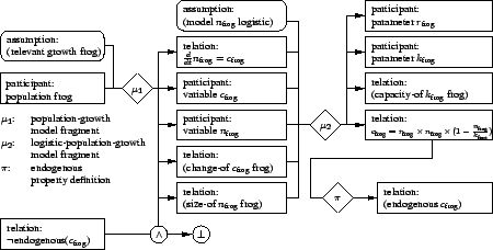To illustrate the model space construction algorithm, Figure 7 presents a small sample model space. It results from the application of the population-growth and logistic-population-growth model fragments and the endogenous property definition, which were described earlier, for a single population ``frog''. If a larger scenario involving multiple populations and relations between these populations were specified, a similar partial model space would be generated for each individual population.