


Next: Analyzing the number of
Up: Positive closed form solution
Previous: Positive closed form solution
Contents
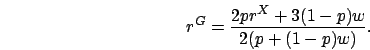
Figure 2.15:
An implementation of the Positive solution,
defined for a distribution
![\begin{figure}\begin{center}
\begin{tabular}[hbt]{\vert l\vert}\hline
($n$, $p$,...
...\mu_1^X$, $\mu_2^X$, $\mu_3^X$)\\
\hline
\end{tabular}
\end{center}\end{figure}](img427.png) |
The Positive solution is defined for almost all the input distributions in  .
Specifically, it is defined for all the distributions in
.
Specifically, it is defined for all the distributions in
Figure 2.15 shows an implementation of the Positive solution.
Below, we elaborate on the Positive solution, and prove an upper bound
on the number of phases used in the Positive solution.
When the input distribution  is in
is in
 ,
the EC distribution produced by the Minimal solution does not have a mass probability at zero.
When is in
,
the EC distribution produced by the Minimal solution does not have a mass probability at zero.
When is in
 ,
can be well-represented by a two-phase Coxian
,
can be well-represented by a two-phase Coxian PH distribution,
whose parameters are given by (2.4)-(2.5).
Below, we focus on input distributions
PH distribution,
whose parameters are given by (2.4)-(2.5).
Below, we focus on input distributions
 .
.
We first consider the first approach of using a mixture of an EC distribution
(with no mass probability at zero),  , and an exponential distribution,
  ,
(i.e.
,
(i.e.
 ).
Let
).
Let
Given a distribution
 ,
we seek
,
we seek  ,
,  ,
,  , and
, and  such that
 |
 |
 |
(2.9) |
 |
 |
 |
(2.10) |
 |
|
 |
(2.11) |
 |
|
 |
(2.12) |
Note that (2.9)-(2.10) guarantee that
we can find, via the Complete solution, an ( )-phase EC distribution, ,
such that has no mass probability at zero and has normalized moments and .
Let be the exponential distribution with
)-phase EC distribution, ,
such that has no mass probability at zero and has normalized moments and .
Let be the exponential distribution with
 .
(2.11)-(2.12) guarantee that,
by choosing
.
(2.11)-(2.12) guarantee that,
by choosing  appropriately,
is well-represented by a distribution
appropriately,
is well-represented by a distribution  , where
The following lemma provides conditions on the input distribution
for which the first approach is defined.
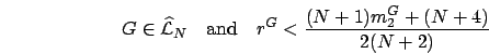
Lemma 5
Suppose
for  (see Figure 2.16(a)).
Let
Then, , , and
conditions (2.9)-(2.12) are satisfied.
(see Figure 2.16(a)).
Let
Then, , , and
conditions (2.9)-(2.12) are satisfied.
A proof of Lemma 5 is postponed to Appendix A.
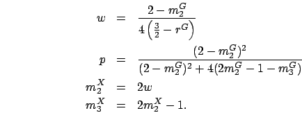
Figure 2.16:
Two regions in  that input can fall into under the Positive solution:
(a) is well-represented by a mixture of an EC distribution and an exponential distribution ;
(b) is well-represented by the convolution of an EC distribution and an exponential distribution
that input can fall into under the Positive solution:
(a) is well-represented by a mixture of an EC distribution and an exponential distribution ;
(b) is well-represented by the convolution of an EC distribution and an exponential distribution  .
.
|
|
The key idea behind Lemma 5 is to fix some of the
parameters so that the set of equations becomes simpler and yet there
exists a unique solution. The difficulty in finding closed form
solutions is that we are given a system of nonlinear equations with
high degree (2.10)-(2.12), and the solutions are not unique. By fixing some of the
parameters, the system of equations can be reduced to have a unique
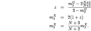
solution. We find
that  given by Lemma 5 has nice characteristics. First,
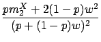
leads to a very simple expression:
given by Lemma 5 has nice characteristics. First,
leads to a very simple expression:  .
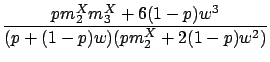
Second, with this expression of ,
the expression involving
.
Second, with this expression of ,
the expression involving  is significantly simplified:
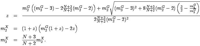
Now, solving (2.10)-(2.12) for  and is a relatively easy task,
and and immediately gives and . Although
Lemma 5 allows us to find a simple closed form
solution, the set of input distributions defined for
Lemma 5 is rather small. This necessitates the
second approach of using the convolution of an EC distribution and an
exponential distribution. Note that the second approach alone does
not suffice, either. Applying the first approach to a small set of
input distributions and applying the second approach to the rest of
the input distribution, in fact, lead to simpler
closed form solutions by both approaches.
and is a relatively easy task,
and and immediately gives and . Although
Lemma 5 allows us to find a simple closed form
solution, the set of input distributions defined for
Lemma 5 is rather small. This necessitates the
second approach of using the convolution of an EC distribution and an
exponential distribution. Note that the second approach alone does
not suffice, either. Applying the first approach to a small set of
input distributions and applying the second approach to the rest of
the input distribution, in fact, lead to simpler
closed form solutions by both approaches.
Next, we consider the second approach of using the convolution of an EC distribution
(with mass probability at zero) and an exponential distribution
(i.e.
 ).
Given a distribution
(we assume
).
Given a distribution
(we assume
 ),
we seek , , and
),
we seek , , and  such that
 |
 |
|
(2.13) |
|
|
 |
(2.14) |
|
|
 |
(2.15) |
|
|
 |
(2.16) |
Note that (2.13)-(2.14) guarantees that
we can find, via the Complete solution, an ()-phase EC distribution, ,
such that has no mass probability at zero and has normalized moments and .
Let be the exponential distribution whose first moment is
 , where is the first moment of .
(2.15)-(2.16) guarantee that,
by choosing appropriately,
is well-represented by the convolution of and .
, where is the first moment of .
(2.15)-(2.16) guarantee that,
by choosing appropriately,
is well-represented by the convolution of and .
The following lemma provides conditions on the input distribution
for which the second approach is defined.
Lemma 6
Suppose
for (see Figure 2.16(b)).
If  , we choose
If
, we choose
If  , we choose
Then, and
conditions (2.13)-(2.16) are satisfied.
, we choose
Then, and
conditions (2.13)-(2.16) are satisfied.
A proof of Lemma 6 is postponed to Appendix A.
Next: Analyzing the number of
Up: Positive closed form solution
Previous: Positive closed form solution
Contents
Takayuki Osogami
2005-07-19
![\includegraphics[width=0.7\linewidth]{fig/PositiveIdea1.eps}](img451.png)
![\includegraphics[width=0.7\linewidth]{fig/PositiveIdea2.eps}](img452.png)