Our goal is to compute a tight upper bound on the likelihood
of the observed findings: ![]() .
As discussed in Section 4.2, we obtain an upper
bound on
.
As discussed in Section 4.2, we obtain an upper
bound on ![]() by introducing upper bounds for individual
node conditional probabilities. We represent this upper bound
as
by introducing upper bounds for individual
node conditional probabilities. We represent this upper bound
as ![]() , which is a product across the individual
variational transformations and may contain contributions due
to findings that are being treated exactly (i.e., are not
transformed). Marginalizing across d we obtain a bound:
, which is a product across the individual
variational transformations and may contain contributions due
to findings that are being treated exactly (i.e., are not
transformed). Marginalizing across d we obtain a bound:
![]()
It is this latter quantity that we wish to minimize with
respect to the variational parameters ![]() .
.
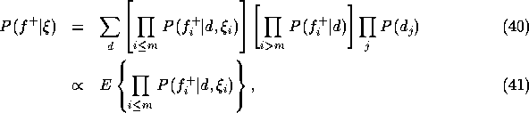
To simplify the notation we assume that the first m positive
findings have been transformed (and therefore need to be
optimized) while the remaining conditional probabilities will be
treated exactly. In this notation ![]() is given by
is given by
where the expectation is taken with respect to the posterior distribution for the diseases given those positive findings that we plan to treat exactly. Note that the proportionality constant does not depend on the variational parameters (it is the likelihood of the exactly treated positive findings). We now insert the explicit forms of the transformed conditional probabilities (see Eq. (17)) into Eq. (41) and find:
where we have simply converted the products over i into sums in the exponent and pulled out the terms that are constants with respect to the expectation. On a log-scale, the proportionality becomes an equivalence up to a constant:
![]()
Several observations are in order. Recall that ![]() is the
conjugate of the concave function f (the exponent), and is therefore
also concave; for this reason
is the
conjugate of the concave function f (the exponent), and is therefore
also concave; for this reason ![]() is convex. In
Appendix C we prove that the remaining term:
is convex. In
Appendix C we prove that the remaining term:
![]()
is also a convex function of the variational parameters.
Now, since any sum of convex functions is convex, we conclude
that ![]() is a convex function of the variational
parameters. This means that there are no local minima in our
optimization problem. We may safely employ the standard
Newton-Raphson procedure to solve
is a convex function of the variational
parameters. This means that there are no local minima in our
optimization problem. We may safely employ the standard
Newton-Raphson procedure to solve ![]() .
Alternatively we can utilize fixed-point iterations. In particular,
we calculate the derivatives of the variational form and
iteratively solve for the individual variational parameters
.
Alternatively we can utilize fixed-point iterations. In particular,
we calculate the derivatives of the variational form and
iteratively solve for the individual variational parameters
![]() such that the derivatives are zero. The derivatives
are given as follows:
such that the derivatives are zero. The derivatives
are given as follows:
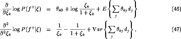
where the expectation and the variance are with respect to the
posterior approximation ![]() , and both derivatives can be
computed in time linear in the number of associated diseases for the
finding. The benign scaling of the variance calculations comes from
exploiting the special properties of the noisy-OR dependence and the
marginal independence of the diseases.
, and both derivatives can be
computed in time linear in the number of associated diseases for the
finding. The benign scaling of the variance calculations comes from
exploiting the special properties of the noisy-OR dependence and the
marginal independence of the diseases.
Calculating the expectations in Eq. (7) is exponentially costly in the number of exactly treated positive findings. When there are a large number of positive findings, we can have recourse to a simplified procedure in which we optimize variational parameters after having transformed all or most of the positive findings. While the resulting variational parameters are suboptimal, we have found in practice that the incurred loss in accuracy is typically quite small. In the simulations reported in the paper, we optimized the variational parameters after approximately half of the exactly treated findings had been introduced. (To be precise, in the case of 8, 12 and 16 total findings treated exactly, we optimized the parameters after 4, 8, and 8 findings, respectively, were introduced).